Magnetic order in the Shastry-Sutherland model

Abstract

The ground state properties of the Shastry-Sutherland model in the presence of an external field are investigated by means of variational states built up from unpaired spins (monomers) and singlet pairs of spins (dimers). The minimum of the energy is characterized by specific monomer-dimer configurations, which visualize the magnetic order in the sectors with fixed magnetization $M=S/N$. A change in the magnetic order is observed if the frustrating coupling $\alpha$ exceeds a critical value $\alpha_{c}(M)$, which depends on $M$. Special attention is paid to the ground state configurations at $M=1/4,1/6,1/8$.

]

I Introduction

The Shastry-Sutherland model[1] defined by the two-dimensional spin 1/2 Hamiltonian

$$H = \sum_{\langle{\bf x},{\bf y}\rangle}{\bf S}({\bf x}){\bf S}({\bf y})+\alpha\sum_{\langle\langle{\bf x},{\bf y}\rangle\rangle}{\bf S}({\bf x}){\bf S}({\bf y})$$ (1)

with nearest neighbor couplings and frustrating next-nearest neighbor couplings on the diagonals shown in Fig. 1 has attracted a lot of interest for theoretical and experimental reasons:

FIG. 1.: The couplings in the Shastry-Sutherland model. Nearest and next-nearest neighbor couplings are represented by dotted and solid lines.

(1) The product wave function

$$\Psi = \prod_{\langle\langle{\bf x},{\bf y}\rangle\rangle}[{\bf x},{\bf y}]$$ (2)

built up from singlet states

$$[{\bf x},{\bf y}] = \frac{1}{\sqrt{2}}\left(\chi_{+}({\bf x})\chi_{-}({\bf y})-\chi_{-}({\bf x})\chi_{+}({\bf y})\right)$$ (3)

is known to be an eigenstate of the Hamiltonian (1), which turns out to be the ground state, if the coupling $\alpha$ exceeds a critical value $\alpha_{c}$ ($\alpha_{c}\approx 1.4$). [2] The phase diagram has been studied recently by Weihong, Oitmaa and Hamer [3] by means of series expansions.

(2) The Hamiltonian (1) is suggested to be an appropriate model for the compound $SrCu_{2}(BO_{3})_{2}$ the magnetic properties of which have been investigated in recent high magnetic field experiments.[4, 5, 6] Plateaus have been found in the magnetization curve $M=M(B)$ at rational values of the magnetization $M/M_{S}=1/3,\,1/4,\,1/8$, where $M_{S}=1/2$ is the saturating magnetization.

From the theoretical point of view the appearance of magnetization plateaus is well understood in quasi one-dimensional systems, e.g. with ladder geometry. [7] Here, a quantization rule has been formulated by Oshikawa, Yamanaka and Affleck, [8] which originates from the prediction of soft modes [9] based on the Lieb-Schultz-Mattis (LSM) theorem. [10] Only the position of the possible plateaus – i.e. the quantized value of the magnetization – are predicted by this rule. The upper and lower critical fields which define the width of the plateau, however, depend on the magnitude of transition matrix elements with a momentum transfer corresponding to the relevant soft mode. These matrix elements contribute to the dynamical and static structure factors and a strong peak in these quantities at the soft mode momenta is needed for a pronounced plateau in the magnetization curve. [9]

The extension of the Lieb Schultz Mattis construction to higher dimensions ($D>1$) meets difficulties. As was pointed out by Oshikawa [11] magnetization plateaus are possible in higher dimensions as well, provided that the “commensurability condition” is satisfied. Based on a topological argument he shows, that this condition is a robust non-perturbative constraint.

The emergence of magnetization plateaus in a modified Shastry-Sutherland model has been discussed in Ref. [[12]]. Recently, Misguich, Jolicœr, and Girvin studied the emergence of magnetization plateaus in the framework of a Chern-Simons theory.[13]

In Ref. [[4]] Kageyama et al. proposed that product wave functions of the type (2) with certain distributions of $N_{S}$ singlets (3) and $N_{T}$ triplets

$$\{{\bf x},{\bf y}\} = \chi_{+}({\bf x})\chi_{+}({\bf y})$$ (4)

might yield an appropriate ansatz for the ground state in the sector with total spin

$$S_{T} = N_{T}/4$$ (5)

where $N_{T}$ and $N_{S}$ are constrained by the total number of sites

$$N_{S}+N_{T} = N/2\,.$$ (6)

Typical examples of these states are shown in Figs. 2(b), 3(b), 4(c) and 4(d). An effective Hamiltonian, describing the interaction between singlets and triplets, has been developed and evaluated in Refs. [[14, 15]].

In this paper, we investigate a wider class of product wave functions - which we call monomer-dimer configurations [16] - and which are aimed to describe the magnetic order at those magnetizations ($M=1/4,1/6,1/8,1/16$), where plateaus are expected. Indeed we find a change in the magnetic order if the frustration parameter exceeds a critical value $\alpha_{c}(M)$, which depends on the magnetization $M$. For $\alpha>\alpha_{c}(M)$ we recover the singlet-triplet configurations proposed in Ref.[[4]]. For $\alpha<\alpha_{c}(M)$, however, we find new configurations with lower energy.

The outline of the paper is as follows: In Sec. II we define the monomer-dimer configurations. In Sec. III we minimize the expectation value of the Hamiltonian (1) between monomer-dimer configurations. This procedure singles out specific configurations, which visualize the magnetic order at fixed magnetization $M$. In Sec. IV we introduce the “frozen monomer approximation”, which allows to lower the energy expectation values between monomer-dimer configurations without changing the magnetic order, i.e. the distribution of “frozen” monomers.

The quality of the frozen monomer approximation is studied for $M=1/8,1/6,1/4$ in Sec. V by a comparison with the ground state energies obtained from exact diagonalizations on finite clusters.

We also look for the formation of magnetization plateaus. Possible interpretations of the observed plateaus in $SrCu_{2}(BO_{3})_{2}$ are discussed in Sec. VI.

II Monomer-Dimer configurations

The Shastry-Sutherland Hamiltonian (1) conserves the total spin

$${\bf S} = \sum_{\bf x}{\bf S}({\bf x})$$ (7)

and we therefore start from eigenstates of

$${\bf S}^{2} = S(S+1)\quad\mbox{and}\quad S_{3}\,=\,-S,\ldots,S\,.$$ (8)

Following Hulth en [17], these states $|K,\nu=2S\rangle$ can be constructed in the sector with total spin $S$ -i.e. magnetization $M=S/N$- as product states of

• unpaired spin-up states at sites ${\bf x}_{1},\ldots,{\bf x}_{\nu}$, $\nu=2S$:

  $$|{\bf x}+\rangle = \chi_{+}({\bf x})$$ (9)

  which we call “monomers”

• singlets of paired spins $[{\bf x},{\bf y}]$ (3) at sites ${\bf x}$, ${\bf y}$ (“dimers”):

  $$|K,\nu\rangle = \prod_{j=1}^{\nu=2S}|{\bf x}_{j}+\rangle\prod_{\langle{\bf x},{\bf y}\rangle}[{\bf x},{\bf y}]$$ (10)

Note, that in the monomer-dimer configuration $K$ each site ${\bf x}$ is occupied exactly once: either by a monomer or a dimer. Moreover, monomer-dimer configurations $|K,\nu\rangle$ yield an overcomplete non-orthogonal set of eigenstates with total spin $S$.

The expectation value of the Hamiltonian (1) between monomer-dimer configurations can be easily calculated with the following rules:

$$\langle 1+,2+|{\bf S}(1){\bf S}(2)|1+,2+\rangle = \frac{1}{4}$$ (11)

$$\langle[1,2]|{\bf S}(1){\bf S}(2)|[1,2]\rangle = -\frac{3}{4}$$ (12)

$$\langle[1,3]2+|{\bf S}(1){\bf S}(2)|[1,3]2+\rangle = 0$$ (13)

$$\langle[1,3][2,4]|{\bf S}(1){\bf S}(2)|[1,3][2,4]\rangle = 0\,.$$ (14)

If we count on each configuration the numbers

• $N_{1}^{(0)}(K)$ of nearest neighbor dimers

• $N_{2}^{(0)}(K)$ of next-nearest neighbor dimers (corresponding to Fig. 1)

• $N_{1}^{(1)}(K)$ of nearest neighbor monomer pairs

• $N_{2}^{(1)}(K)$ of next-nearest neighbor monomer pairs (corresponding to Fig. 1)

we can immediately compute the expectation value:

$$\langle K,\nu|H|K,\nu\rangle = -\frac{3}{4}N_{1}^{(0)}-\frac{3}{4}\alpha N_{2}^{(0)}$$ (16)

$$+\frac{1}{4}N_{1}^{(1)}+\frac{\alpha}{4}N_{2}^{(1)}\,.$$

In order to minimize this expectation value we have to look for configurations with

• a maximum number of nearest neighbor dimers $N_{1}^{(0)}$ if $\alpha<1$

• a maximum number of next-nearest neighbor dimers $N_{2}^{(0)}$ if $\alpha>1$

• a minimum number of monomer pairs $N_{1}^{(1)}$, $N_{2}^{(1)}$ on nearest and next-nearest neighbor sites.

III Magnetic ordering at fixed magnetizations

A $M=1/4$, $\nu=N/2$

Let us start with $M=1/4$. In this situation we have to distribute $\nu=N/2$ monomers and $N/4$ dimers on the square lattice. We cannot avoid the appearance of monomer pairs on nearest and next-nearest neighbor sites, but we can minimize their numbers $N_{1}^{(1)}$ and $N_{2}^{(1)}$ if we cover the lattice in the way shown in Fig.2(a). The bold lines symbolize the nearest-neighbor singlets, the thin lines the monomer pairs on nearest and next-nearest neighbor sites. Dimer pairs can interact via the next-nearest neighbor couplings in the Hamiltonian; they are represented by dotted lines. According to (16), the expectation value of the Hamiltonian is found to be:

$$E(K_{1},1/4) = \langle K_{1},N/2|H|K_{1},N/2\rangle$$ (17)

$$= \frac{N}{8}(-1+\alpha/4)\,.$$ (18)

A second configuration, shown in Fig. 2(b) has been proposed in Ref.[[5]] as a possible ground state configuration for $M=1/4$. In this case, the expectation value of $H$ turns out to be:

$$E(K_{2},1/4) = \langle K_{2},N/2|H|K_{2},N/2\rangle$$ (19)

$$= -\alpha\frac{N}{8}\,.$$ (20)

FIG. 2.: Monomer-dimer configurations with minimal energy expectation value at $M=1/4$. Bold lines represent “dimers” i.e. paired spins coupled to singlets. Dotted lines indicate the couplings between dimers induced by Hamiltonian (1). Unpaired spin-up states (“monomers”) [Eq.(9)] are symbolized by solid points; their couplings on nearest and next-nearest neighbor sites are indicated by thin lines. (a) configuration $K_{1}$ for $\alpha<\alpha_{c}(M=1/4)=4/5$; (b) configuration $K_{2}$ for $\alpha>\alpha_{c}(M=1/4)$

The difference of (17) and (19)

$$E(K_{1},1/4)-E(K_{2},1/4) = \frac{N}{8}(-1+\frac{5}{4}\alpha)$$ (21)

changes its sign for $\alpha=4/5$, which means there is a change in the magnetic order from configuration $K_{1}$ to $K_{2}$ if the frustration parameter exceeds the value $\alpha_{c}(M=1/4)=4/5$.

B $M=1/6$, $\nu=N/3$

Next, we turn to the case $M=1/6$, where we have to distribute $\nu=N/3$ monomers and $N/3$ dimers on the lattice. The configuration $K_{1}$ [Fig. 3(a)] minimizes the number $N_{2}^{(1)}$ of monomer pairs on next-nearest neighbor sites, whereas in the configuration $K_{2}$ [Fig. 3(b)] the next-nearest neighbor sites of Fig. 1 are occupied with singlets and triplets in the spirit of Ref.[[5]]. The difference of the expectation values of $H$

$$E(K_{1},1/6) = \langle K_{1},N/3|H|K_{1},N/3\rangle$$ (23)

$$= -\frac{N}{4}(1-\frac{\alpha}{12})$$ (24)

$$E(K_{2},1/6) = \langle K_{2},N/3|H|K_{2},N/3\rangle$$ (25)

$$= -\frac{N}{4}\frac{5\alpha}{6}$$ (26)

$$E(K_{1},1/6)-E(K_{2},1/6) = -\frac{N}{4}(1-\frac{11}{12}\alpha)$$ (27)

changes sign for $\alpha_{c}(M=1/6)=12/11$. Again we observe a change in the magnetic order from $K_{1}$ to $K_{2}$ if $\alpha$ passes this value.

FIG. 3.: Same as Fig.2 for $M=1/6$: (a) configuration $K_{1}$ $\alpha<\alpha_{c}(M=1/6)=12/11$; (b) configuration $K_{2}$ for $\alpha>\alpha_{c}(M=1/6)$

It is remarkable to note, that in both cases $\alpha<\alpha_{c}(M=1/6)$ and $\alpha>\alpha_{c}(M=1/6)$ a stripe order of the monomers is predicted.

C $M=1/8$, $\nu=N/4$

In the case of $M=1/8$ we have to distribute $\nu=N/4$ monomers and $3N/8$ dimers on the square lattice. We can avoid now completely the appearance of monomer pairs on nearest and next-nearest neighbor sites as is demonstrated by the configuration $K_{1}$ shown in Fig. 4(a). Owing to the stripe structure, we can also construct a second configuration [Fig. 4(b)] with $N_{1}^{(0)}=N/8$ dimers on nearest neighbor sites and $N_{2}^{(0)}=N/4$ dimers on next-nearest neighbor sites. Two further configurations $K_{3}$ and $K_{4}$ have been proposed in Refs. [[5, 15]], which only contain $N_{1}^{(0)}=3N/8$ dimers and $N_{1}^{(1)}=N/8$ monomer pairs on next-nearest neighbor sites.

The corresponding energy expectation values are

$$E(K_{1},1/8) = -\frac{9}{32}N$$ (29)

$$E(K_{2},1/8) = -\frac{3}{32}N(1+2\alpha)$$ (30)

$$E(K_{3},1/8) = E(K_{4},1/8)=-\frac{N}{4}\alpha\,.$$ (31)

Comparing the expectation values (29)-(31) we expect a change in the magnetic order with $\alpha$:

FIG. 4.: Same as Fig.2 for $M=1/8$: (a) configuration $K_{1}$, $\alpha<1$; (b) configuration $K_{2}$, $1<\alpha<3/2$; (c) and (d) configurations $K_{3}$ and $K_{4}$, $\alpha>3/2$

$$\alpha<1:\quad E(K_{1})<E(K_{2})<E(K_{3})=E(K_{4})$$ (32)

$$1<\alpha<\frac{3}{2}: E(K_{2})<E(K_{1})<E(K_{3})=E(K_{4})$$ (33)

$$\frac{3}{2}<\alpha:\quad E(K_{3})=E(K_{4})<E(K_{2})<E(K_{1})\,.$$ (34)

IV The frozen monomer approximation (FMA)

The monomer-dimer configurations which we developed in the last section to describe the magnetic order in the Shastry-Sutherland model are not eigenstates of the Hamiltonian (1). Application of (1) onto these states will generate new states. In this section we study the impact of those couplings in the Hamiltonian, which generate interactions only between dimer pairs, i.e. we consider an approximation where the $\nu$ monomers are frozen at sites ${\bf x}_{1}\ldots{\bf x}_{\nu}$ in the configuration $|K,\nu\rangle$. For each of these configurations, we define a decomposition of the Hamiltonian in three parts:

$$H = H_{\nu}+H(K)+\sum_{i}H({\bf x}_{i},K)$$ (35)

where

• $H_{\nu}$ contains all the nearest and next-nearest neighbor couplings between the sites ${\bf x}_{1}\ldots{\bf x}_{\nu}$, where the monomers are located. All other sites are occupied with dimers. They form an antiferromagnetic cluster $K$, which are represented by the dimers and the dotted connections between dimers in Figs. 2(a)-4(d).

• The cluster Hamiltonians $H(K)$ is defined by the nearest and next-nearest neighbor couplings on the dimer cluster $K$.

• The nearest and next-nearest neighbor couplings in $H({\bf x}_{i},K)$ take into account the remaining interactions between the monomer at site ${\bf x}_{i}$ and the dimers in the cluster $K$.

The ground state energy $E(K)$ of the antiferromagnetic cluster Hamiltonian $H(K)$

$$H(K)\Psi(K) = E(K)\Psi(K)\,.$$ (36)

is obviously lower than the expectation value of $H(K)$ between the dimer product wave function on the cluster $K$.

The product ansatz

$$|{\bf x}_{1}\ldots{\bf x}_{\nu},K\rangle = \prod_{i=1}^{\nu=2S}|{\bf x}_{i}+\rangle\prod_{j}\Psi(K)$$ (37)

yields an eigenfunction of $H_{\nu}+H(K)$ with energy

$$E(K,\nu) = \frac{1}{4}N_{1}^{(1)}(K)+\frac{\alpha}{4}N_{2}^{(1)}(K)+E(K)\,$$ (38)

which again represents an upper bound for the exact ground state energy $E_{0}(M=\nu/2N)$ of (35) in the sector with magnetization $M=S/N$:

$$E_{0}(M=\nu/2N) \leq E(K,\nu)\,.$$ (39)

In the derivation of (39) one has to use the fact, that the expectation value of the interaction term $H(\nu,K)$ between the product state (37) vanishes, since

$$\langle\Psi(K)|S_{l}(y)|\Psi(K)\rangle = 0\quad y\in K,\,\,l=1,2,3\,.$$ (40)

V Numerical results

In order to check the quality of the frozen monomer approximation (FMA), we have computed the energies (38) and compared with exact diagonalizations of the Shastry-Sutherland Hamiltonian at fixed magnetization $M=\nu/2N$ on lattices with $N=4\times 4=16$ and $N=4\times 6=24$.

The strongest effects due to the frozen monomer approximation occur at small magnetizations. We therefore start with $M=1/8$.

A $M=1/8$

From Fig. 4(a)-4(c) we see that the interactions between the dimers generate a two-dimensional cluster which contains all dimers in the configuration. In contrast, the dimers in Fig. 4(d) form quasi-one-dimensional “stripe” clusters.

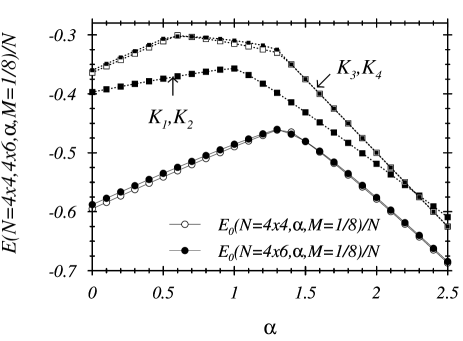
FIG. 5.: Ground state energies per site $E_{0}(N,M,\alpha)/N$ for Shastry-Sutherland lattices of $N=4\times 4,4\times 6$ sites and corresponding FMA energies of configurations $K_{1},...,K_{4}$ at magnetization $M=1/8$.

In Fig. 5 the expectation values $E(K_{j},M=1/8,\alpha)$, $j=1,2,3,4$ in the frozen monomer approximation – corresponding to the configurations Fig. 4(a)-4(d) – are represented by dotted lines.

The following points should be noted:

• The transition in the magnetic order from configuration $K_{2}$ [Fig. 4(b)] to configuration $K_{3}$ [Fig. 4(c)] occurs here at a larger value of the frustration parameter

  $$\alpha_{c}(M=1/8) \simeq 2.3\,.$$ (41)

  At this value the difference in the expectation values $E(K_{1},M=1/8,\alpha)-E(K_{3},M=1/8,\alpha)$ changes sign. For smaller values of $\alpha$ the distribution of monomers according to Fig. 4(a),(b) is favored in comparison with the distribution of triplets in Fig. 4(c),(d).

• For $\alpha>1.3$ the expectation values

  $$E(K_{3},M) = E(K_{4},M)$$ (42)

  corresponding to configurations $K_{3}$ and $K_{4}$ [Fig. 4(c) and Fig. 4(d)] coincide in the frozen monomer approximation. Indeed, here, the dimer product ansatz (10) is an eigenstate of the antiferromagnetic cluster Hamiltonian (36). In other words: The interactions between the dimers [dotted lines in Fig. 4(c),(d)] do not lower the ground state expectation value.

• The expectation values $E(K_{j},M=1/8)$ deviate significantly for $\alpha\leq 1.3$ from the exact results given by the solid curves. Therefore, other distributions of monomers should play an important role in the exact ground state.

• For small $\alpha$, the eact results show a linear behavior which is well reproduced in a perturbative expansion in $\alpha$:

  $$N^{-1}E_{0}(M,\alpha) = \epsilon_{1}(M)+\frac{\alpha}{4}\epsilon_{2}(M)$$ (43)

  where

  $$\epsilon_{j}(M) = \langle 0|{\bf S}({\bf x}){\bf S}({\bf y})|0\rangle\quad j=1,2$$ (44)

  $$\epsilon_{1}(1/8) \simeq -0.59$$ (45)

  $$\epsilon_{2}(1/8) \simeq +0.43$$ (46)

  are the ground state expectation values of the nearest neighbor ($j=1$, $\langle{\bf x},{\bf y}\rangle$) and next-nearest neighbor ($j=2$, $\langle\langle{\bf x},{\bf y}\rangle\rangle$) spin-spin correlators of the unfrustrated Hamiltonian $H(\alpha=0)=H_{1}(1,1)$. [18]

• Finite-size effects are small, as can be seen from a comparison of the exact results for the two systems $N=16$ and $N=24$.

B $M=1/6$

In this case the interactions between the dimers form quasi-one-dimensional clusters with stripe geometry as can be seen from Fig. 3(a),(b). The expectation values $E(K_{j},M=1/6,\alpha)$ $j=1,2$ in the frozen monomer approximation are shown in Fig. 6. The transition point in the magnetic order is found her at

$$\alpha_{c}(M=1/6) = 1.2\,.$$ (47)

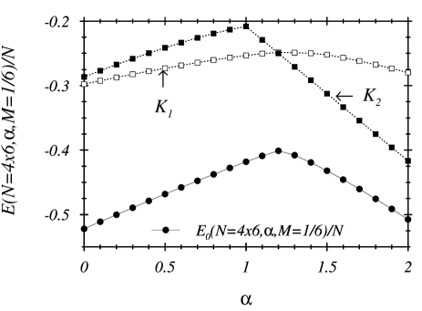
FIG. 6.: Ground state energy per site $E_{0}(N,M,\alpha)/N$ for a Shastry-Sutherland lattice of $N=4\times 6$ sites and corresponding FMA energies of configurations $K_{1},K_{2}$ at magnetization $M=1/6$.

At this point the exact result of the $N=4\times 6=24$ system (solid line) has its maximum. The expectation values $E(K_{j},M=1/6)$ deviate significantly for $\alpha<1.2$ from the exact results given by the solid curve.

C $M=1/4$

The configuration $K_{1}$ in Fig. 2(a) is built up from 4-point singlet clusters. In the frozen monomer approximation we lower the energy if we substitute each dimer pair

FIG. 7.: The 2-dimer cluster in the configuration $K_{1}$ [Fig.2(a)]

$$\hskip 71.13188pt[1,2]\,[3,4] \rightarrow \Psi(1,2,3,4)$$ (48)

by the ground state of the 4-point cluster computed from the 4-point Hamiltonian

$$H(1,2,3,4) = {\bf S}(1){\bf S}(2)+{\bf S}(3){\bf S}(4)+\alpha{\bf S}(2){\bf S}(3)\,.$$ (49)

The corresponding ground state energy

$$E(1,2,3,4) = -\frac{2+\alpha}{4}-\frac{1}{2}\left(4-2\alpha+\alpha^{2}\right)^{1/2}<-\frac{3}{2}\,$$ (50)

is lower than the energy of the dimer pair. Taking into account this effect in the expectation value (17) we find

$$E(K_{1},M=1/4) = -\frac{N}{16}\left(4-2\alpha+\alpha^{2}\right)^{1/2}\,.$$ (51)

Note that there are no interactions between the dimers in the configuration $K_{2}$ [Fig. 2(b)]. Therefore the ground state energy (19) cannot be lowered through the frozen monomer approximation. The energy differences of (51) and (19) changes its sign at

$$\alpha_{c}(M=1/4) = \frac{1}{3}(-1+\sqrt{3})\simeq 0.869\,.$$ (52)

Below this value the expectation value $E(K_{1},M=1/4)$ is a very poor approximation for the exact ground state energy, indicating that the true ground state is not reproduced adequately by the frozen monomer approximation.

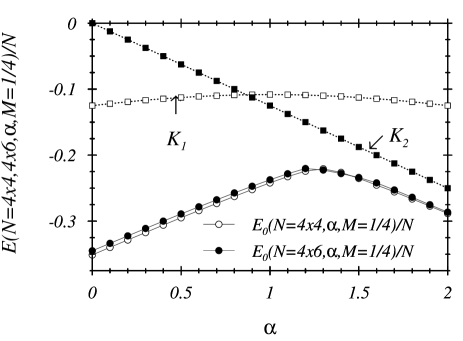
FIG. 8.: Ground state energies per site $E_{0}(N,M,\alpha)/N$ for Shastry-Sutherland lattices of $N=4\times 4,4\times 6$ sites and corresponding FMA energies of configurations $K_{1},,K_{2}$ at magnetization $M=1/4$.

In Fig. 8 we compare the energy expectation values $E(K_{1},M=1/4,\alpha)$ (51) and, $E(K_{2},M=1/4,\alpha)$ (19) with the exact diagonalization on finite systems with $N=4\times 4=16$ and $N=4\times 6=24$ sites. The maximum of the exact ground state energy $E_{0}(M=1/4,\alpha)$ is found at $\alpha\simeq 1.5$ far beyond the transition point (52) from configuration $K_{1}$ to $K_{2}$.

We have also studied the formation of plateaus in the magnetization curve at $M=1/8,1/6,1/4$ by exact diagonalizations on the finite clusters with $N=4\times 4=16$ and $N=4\times 6=24$ sites. The lower and upper critical fields

$$B_{L}(M,\alpha) = E_{0}(M,\alpha)-E_{0}(M-2/N,\alpha)$$ (53)

$$B_{U}(M,\alpha) = E_{0}(M+2/N,\alpha)-E_{0}(M,\alpha)$$ (54)

were computed from ground state energies $E_{0}(M-2/N,\alpha)$, $E_{0}(M,\alpha)$, $E_{0}(M+2/N,\alpha)$ with neighboring total spins $S-1,S,S+1$, $S=M\cdot N$. The results are shown in Fig. 9 (a) for $M=1/8$ (b) for $M=1/6$ (c) for $M=1/4$.

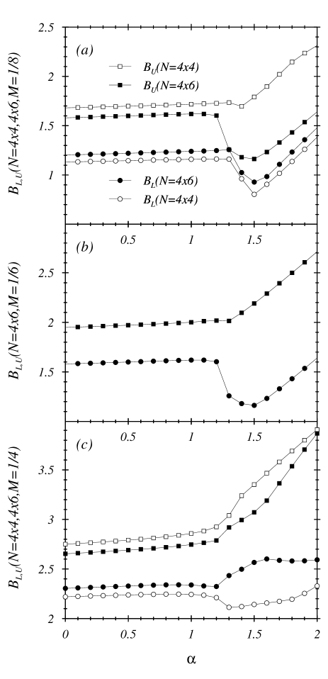
FIG. 9.: Upper($B_{U}$) and lower($B_{L}$) critical fields for magnetizations $M=1/8$ (a), $1/6$ (b), $1/4$ (c) calculated on Shastry-Sutherland lattices of $N=4\times 4$ (a,c) and $N=4\times 6$ (a-c) sites.

For $\alpha<1.2$ all critical fields are rather $\alpha$-independent. The finite-size effects indicate that the plateau width

$$\Delta(M,\alpha) = B_{U}(M,\alpha)-B_{L}(M,\alpha)\quad\mbox{for }\alpha<1.2$$ (55)

will vanish in the thermodynamic limit $N\rightarrow\infty$ as it is known for the unfrustrated model ($\alpha=0$).

For $\alpha=1.5$ the lower critical fields $B_{L}(M=1/8,\alpha)$ and $B_{L}(M=1/6,\alpha)$ have a pronounced minimum; beyond this value ($\alpha>1.5$) all lower and upper critical fields for $M=1/8,1/6$ increase with $\alpha$.

For $M=1/8$ [Fig. 9(a)] and $\alpha>1.5$, finite-size effects appear to be small for $B_{L}(M=1/8,\alpha)$ but large for $B_{U}(M=1/8,\alpha)$. We suggest that the rectangular geometry of the $4\times 6$ system might be responsible for this failure. It breaks the rotational invariance and therefore does not allow for the rotated patterns in Fig. 4.

For $M=1/4$ [Fig. 9(c)] and $\alpha>1.5$ we observe a rather clean signal for the opening of a magnetization plateau.

VI Discussion and perspectives

In this paper, we have investigated the magnetic order of the Shastry-Sutherland model at fixed magnetizations $M=1/8,1/6,1/4$. For large enough values of the frustration parameter

$$\alpha>\alpha_{c}(M=1/8)=2.3, \alpha>\alpha_{c}(M=1/6)=1.2,$$ (56)

$$\alpha>\alpha_{c}(M=1/4)=0.89$$ (57)

configurations built up from singlets and triplets on the Shastry-Sutherland lattice [cf. Figs. 2(b), 3(b), 4(c),(d)] – as they were proposed in [[4, 5, 14]] – yield the lowest energy expectation values. Here, a strong coupling approach ($\alpha^{-1}\rightarrow 0$) to take into account singlet-triplet interactions is applicable. With this method Momoi and Totsuka [14] found evidence for plateaus in the magnetization curve at $M=1/4$ and $M=1/6$. However, they did not find plateaus at smaller magnetizations ($M=1/8$ and $M=1/16$), “since the mechanism to stabilize these plateaus is not yet clear” – as they say.

We think that this failure has a simple explanation: The singlet-triplet configurations on the Shastry-Sutherland lattice (cf. e.g. Fig. 4(c),(d) for $M=1/8$) are unfavorable, since the formation of triplets on next-nearest neighbor sites costs energy [cf. e.g. (16)]. Configurations – like $K_{2}$ in Fig. 4(b) for $M=1/8$ – with well separated monomers (unpaired spin-up states) yield a lower energy as long as $\alpha$ is not too large ($\alpha<\alpha_{c}(M=1/8)=2.3$).

If the coupling $\alpha$ – realized in the compound $SrCu_{2}(BO_{3})_{2}$ – is indeed below this value, the experimentally observed plateaus at $M=1/8$ and $M=1/16$ cannot be associated with singlet-triplet configurations on the Shastry-Sutherland lattice.

In order to find the correct magnetic order at low magnetizations $M<\nu/2N$ and $\alpha<2.3$ a more general ansatz for the ground state configurations is needed. This can be constructed in terms of monomers at fixed sites ${\bf x}_{1}\ldots{\bf x}_{\nu}$. The spins on the remaining sites form an antiferromagnetic cluster, the ground state energy of which depends on the fixed positions of the $\nu$ monomers. Therefore, a specific distribution of monomers characterizing the magnetic order is given by a minimum of the ground state energy of the corresponding antiferromagnetic cluster (cf. e.g. Fig. 4(a),(b) for $M=1/8$). We expect that for small values of $M$ – in particular in the sectors with a finite number $\nu$ of monomers, i.e. $M=\nu/2N\rightarrow 0$ for $N\rightarrow\infty$ – the singlet-triplet configurations on the Shastry-Sutherland lattice are dominant again (for $\alpha\geq\alpha_{c}(M=0)=1.4$). Each of the $(N-\nu)/2$ singlets lowers the energy by $-3\alpha/4$ whereas each of the few ($\nu/2$) triplets costs energy $\alpha/4$.

It should also be noted that the frozen monomer approximation becomes better and better for $M\rightarrow 0$, since the antiferromagnetic clusters cover more and more of the whole lattice.

Finally, we have also studied the formation of plateaus in the magnetization curve of the Shastry-Sutherland model.

We looked for the $\alpha$-dependence of the lower and upper critical fields as they follow from exact diagonalizations on finite clusters with $N=4\times 4=16$ and $N=4\times 6=24$ sites. All the critical fields are almost $\alpha$-independent for $\alpha<1.2$, but change rapidly above this value. Indications for the opening of a plateau are visible for $M=1/4,1/6$ supporting previous results with other methods. [13, 14, 15]

The situation for $M=1/8$ appears to be more subtle. The lower critical field has a pronounced minimum at $\alpha=1.5$. Here, the finite-size effects are rather small. In contrast the upper critical field reveals a strong finite-size dependence. Computations on larger systems are needed for a reliable estimate of the thermodynamic limit.

- [1] B. S. Shastry, B. Sutherland, Physica 108 ,B, 1308 (1981)
- [2] S. Miyahara, K. Ueda, Phys. Rev. Lett. 82, 3701 (1999); Phys. Rev. B 61, 3417 (1999)
- [3] Z. Weihong, J. Oitmaa, C. J. Hamer, cond-mat/0107019
- [4] H. Kageyama et al., J. Phys. Soc. Jpn. 67, 4304 (1998);68, 1821 (1999); Phys. Rev. Lett. 82, 3168 (1999)
- [5] K. Onizuka, H. Kageyama et al., J. Phys. Soc. Jpn. 69, 1016 (2000)
- [6] H. Nojiri et al., J. Phys. Soc. Jpn. 68, 2906 (1999); T. Rõõm et al., Phys. Rev. B 61, 14342 (2000); S: Zherlitsyn et al., Phys. Rev. B 62, R6097 (2000)
- [7] D. C. Cabra, A. Honecker, P. Pujol, Phys. Rev. Lett. 79, 5126 (1997); R. M. Wießner, A. Fledderjohann, K.-H. Mütter, M. Karbach, Phys. Rev. B 60, 6545 (1999); Eur. Phys. J. B 15, 475 (2000)
- [8] M. Oshikawa, M. Yamanaka, and I. Affleck, Phys. Rev. Lett. 78, 1984 (1997)
- [9] A. Fledderjohann, C. Gerhardt, M. Karbach, K.-H. Mütter, and R. Wiessner, Phys. Rev. B 59, 991 (1999)
- [10] E. Lieb, T. Schultz, and D. Mattis, Annals of Phys. 16, 407 (1961)
- [11] M. Oshikawa, Phys. Rev. Lett. 84, 1535 (2000)
- [12] E. Müller-Hartmann, R. R. P. Singh, C. Knetter, G. Uhrig, Phys. Rev. Lett. 84, 1808 (2000)
- [13] G. Misguich, Th. Jolicœur, S. M. Girvin, Phys. Rev. Lett. 87, 097203 (2001)
- [14] T. Momoi, K. Totsuka, Phys. Rev. B 61, 3231 (2000); Phys. Rev. B 62, 15067 (2000)
- [15] Y. Fukumoto, A. Oguchi, J. Phys. Soc. Jpn. 69, 1286 (2000); Y. Fukumoto, cond-mat/0012396
- [16] M. Karbach, K.-H. Mütter, P. Ueberholz, H. Kröger, Phys. Rev. B 48, 13666 (1993)
- [17] L Hulth en, Ark. f. Mat., Astr. o. Fys. 26A, 1 (1938)
- [18] A. Fledderjohann, K.-H. Mütter, subm. to Eur. Phys. J. B (2001)