Threshold Disorder as a Source of Diverse and
Complex Behavior in Random Nets

Abstract

We study the diversity of complex spatio-temporal patterns in the behavior of random synchronous asymmetric neural networks (RSANNs). Special attention is given to the impact of disordered threshold values on limit-cycle diversity and limit-cycle complexity in RSANNs which have ‘normal’ thresholds by default. Surprisingly, RSANNs exhibit only a small repertoire of rather complex limit-cycle patterns when all parameters are fixed. This repertoire of complex patterns is also rather stable with respect to small parameter changes. These two unexpected results may generalize to the study of other complex systems. In order to reach beyond this seemingly-disabling ‘stable and small’ aspect of the limit-cycle repertoire of RSANNs, we have found that if an RSANN has threshold disorder above a critical level, then there is a rapid increase of the size of the repertoire of patterns. The repertoire size initially follows a power-law function of the magnitude of the threshold disorder. As the disorder increases further, the limit-cycle patterns themselves become simpler until at a second critical level most of the limit cycles become simple fixed points. Nonetheless, for moderate changes in the threshold parameters, RSANNs are found to display specific features of behavior desired for rapidly-responding processing systems: accessibility to a large set of complex patterns.

1 Introduction

Random Synchronous Asymmetric Neural Networks (RSANNs) with fixed synaptic coupling strengths and fixed neuronal thresholds/inputs tend to have access to a very limited set of different limit cycles (Amari (1974), Clark, Kürten & Rafelski (1988), Littlewort, Clark & Rafelski (1988), Hasan (1989), Rand, Cohen & Holmes (1988), Clark (1990), Schreckenberg (1992)). We will show here, however, that when we add a moderate amount of randomly quenched noise or disorder, by choosing the neural thresholds or inputs to vary within a prescribed gaussian distribution, we can gain controllable, and we believe biologically relevant, access to a wide variety of limit cycles, each displaying dynamical participation by many neurons.

The appearance of limit-cycle behavior in central pattern generators is evidence for cyclic temporal behavior in biological systems (Hasan (1989), Marder & Hooper (1985)). Previous computational models, as discussed above, do not exhibit a diverse repertoire of limit-cycle behaviors, as biological systems often demonstrate (e.g., the different gaits of a horse, or the different rhythmic steps of a good human dancer). Additonally, it is our belief that the biologically-interesting networks are those in which a significant fraction of the neurons can (and often do) participate in the local dynamics. In principle, spatially-sparse neuronal firing patterns can be constructed from a large network of strongly-participatory neurons by self-organized architectural inhibition of selected neuronal assemblies. This can leave the uninhibited neuronal assemblies able to freely participate in the neural dynamics (for some time), though these uninhibited neurons or neuronal assemblies may be isolated in space from each other, only connected to other active neurons through non-local or indirect connections (Gray & Singer (1990)). Therefore, in this paper, we explore the problem of how to produce a computational neural model which possesses a diverse repertoire of strongly-participatory limit-cycle behaviors.

A system which can access many limit cycles should always be able to access a novel mode; hence the system would have the potential to be a ‘creative’ system. Herein, we demonstrate conditions sufficient to allow a simple computational neural system to access creative dynamical behavior.

In Section 2 we introduce RSANNs along with the concept of threshold disorder, as well as a measure to distinguish different limit cycles. In our quantitative investigations we need to introduce, with some precision, concepts which intuitively are easy to grasp, but which mathematically are somewhat difficult to quantify. We define ‘eligibility’ in Section 3.1 as an entropy-like measure of the fraction of neurons which actively participate in the dynamics of a limit cycle. In order to quantify the RSANN’s accessibility to multiple limit-cycle attractors, we define ‘diversity’ in Section 3.2 as another entropy-like measure, calculated from the probabilities that the RSANN converges to each of the different limit cycles. The difference between eligibility and diversity is that the former applies to a limit cycle observed in a specific network, while the latter applies to the collection of limit cycles that the network can exhibit. To measure the creative potential of a system, we introduce the concept of ‘volatility’ as the ability to access a huge number of highly-eligible cyclic modes. We find that in terms of these diagnostic variables, as the neuronal threshold disorder $\varepsilon$ increases, our RSANN exhibits a phase transformation at $\varepsilon=\varepsilon_{1}$ from a small number to a large number of different accessible limit-cycle attractors (Section 3.2), and another phase transformation at $\varepsilon=\varepsilon_{2}>\varepsilon_{1}$ from high eligibility to low eligibility (Section 3.1). Our main result is that the volatility is high only in the presence of threshold disorder of suitably chosen strength between $\varepsilon_{1}\leq\varepsilon\leq\varepsilon_{2}$, thereby allowing access to a diversity of eligible limit-cycle attractors (Section 3.3).

2 Random asymmetric neural networks with threshold or input noise

Symmetric neural networks (SNNs) (Hopfield (1982)) became widely used in associative memory applications due to their ability to store a large number of patterns as fixed points of their dynamics; however, their dynamical behaviour is restricted to fixed points or limit cycles of period 2. In contrast, asymmetric neural networks (RSANNs) show a complicated dynamical behaviour, including limit cycles of large periods or even chaos (Amari (1974), Clark, Rafelski & Winston (1985), Clark, Kürten & Rafelski (1988), Littlewort, Clark & Rafelski (1988), Kürten (1988), Bressloff & Taylor (1989), Clark (1990, 1991), McGuire, Littlewort & Rafelski (1991), McGuire et al. (1992), Bastolla & Parisi (1997)). Moreover, they offer considerably more biological realism, since real neuronal connections tend to be unidirectional.

We investigate a network of $N$ threshold elements, i.e. their firing states have binary values $x_{i}\in\{0,1\}$. Each neuron $i$ is connected to $M<N$ presynaptic neurons by unidirectional weights $w_{ij}$, with $w_{ij}\neq w_{ji}$ and $w_{ii}=0$. All weights are independent random variables, drawn from a uniform distribution within $[-1,1]$. A neuron fires if its post-synaptic-potential (PSP) is greater than its specific threshold $V_{i}$. Therefore the network is described by the following system of equations for ‘sum-and-fire’ McCullough-Pitts neurons:

$$x_{i}(t+1) =\Theta\bigl{(}\sum_{j=1}^{M}w_{ij}x_{j}(t)-V_{i}\bigr{)}\quad\forall i\in 1,\dots,N\,,$$ (1)

where $\Theta$ is the Heaviside function. Supposing that all neurons should actively participate in the dynamics, with a mean firing rate $\langle x_{i}\rangle=\frac{1}{2}$, the mean thresholds $V^{0}_{i}$ are adjusted so that the mean overall input

$$\langle u_{i}\rangle=\langle\sum w_{ij}x_{j}-V^{0}_{i}\rangle\approx\sum w_{ij}\langle x\rangle-V^{0}_{i}\,$$ (2)

to a generic neuron $i$ becomes zero (so that it is poised on the boundary between firing and not firing). Thus, we have:

$$V^{0}_{i} =\frac{1}{2}\sum_{j}w_{ij},$$ (3)

$$V_{i} =\eta_{i}V_{i}^{0},$$ (4)

where the parameter $\eta_{i}$ is chosen to modulate the threshold. The case $\eta_{i}\equiv 1$ for all $i$ corresponds to the choice known as ‘normal’ thresholds (Clark (1991)). The mean firing rate of 0.5 is quite high biologically, but computationally, it is a reasonable point to begin our research; it is not too difficult to adapt the treatment to lower mean firing rates. In order for a given amount of threshold disorder to affect all neurons more-or-less equally, we have chosen here a multiplicative scaling of the thresholds relative to the normal thresholds rather than an additive scaling. We do not consider synaptic noise or modulation; hence the weights $w_{ij}$ are kept fixed for a given network.

In considering the living neural networks in the brain, some researchers treat the neuronal thresholds as constant and noiseless (as in the Hodgkin-Huxley and Fitzhugh-Nagumo models; see Murray (1989) for a summary); others are convinced that neurons live in a very noisy environment, both chemically and electrically, with nontrivial consequences for neuronal and network function (see Zador (1997), Chow & White (1996), Clark (1988), Buhmann & Schulten (1987), Shaw & Vasudevan (1974), Little (1974), Taylor (1972), and Lecar & Nossal (1971)). Examining the issue more closely, we may note that Mainen & Sejnowski (1995) have presented data suggesting a low intrinsic noise level for neurons, which does not seriously affect the precision of spike timing in the case of stimuli with fluctations resembling synaptic activity. On the other hand, Pei, Wilkens & Moss (1996) have presented evidence that noise can exert beneficial effects on neural processing through the phenomenon of stochastic resonance.

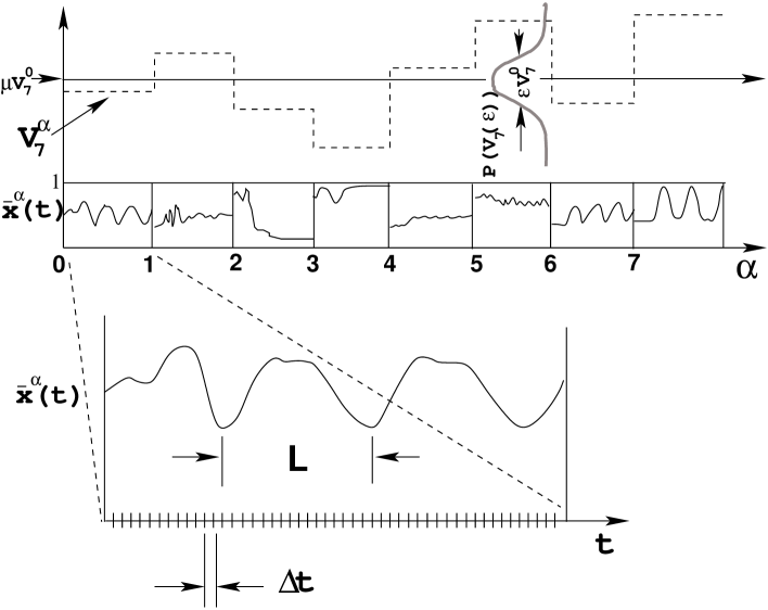
Figure 1: Qualitative sketch showing the varying threshold for neuron #7 ($V_{7}^{\alpha}$) and the spatially-averaged firing rate $\bar{x}^{\alpha}(t)$, as a function of trial-number $\alpha$, and in the inset, a magnified view of $\bar{x}^{\alpha}(t)$, all as functions of time, $t$.

Mathematically, the external inputs to a neuron from sensory organs or from other areas of the neural system can also be treated as a modulation of the threshold of that neuron. This suggests that the results obtained on threshold modulation might be easily generalized to the situation of external modulation.

Taken together, the noisiness of thresholds and the variability of inputs can be viewed as a changing environment. We simply model this complex changing environment by varying the normal thresholds using multiplicative gaussian noise $\eta_{i}$ with mean $\mu=1$ and standard deviation $\varepsilon$, leading to Eq. 4. The components $\eta_{i}$ are chosen independently for all neurons $i$. It may be much more reasonable to consider spatially-correlated noise amplitudes, but such a study exceeds the scope of our present effort.

2.1 Limit-Cycle Search

Since we wish to study the diversity of different limit cycles accessible with small changes of the thresholds, we need a robust criterion for detecting limit cycles. Even in the presence of small-amplitude noise effective on a shorter time scale than the cycle length, the neural net will never stabilize into a detectable perfect cycle. Rather, it will either converge to an approximate limit cycle with occasional misfirings or never converge at all. Such approximate limit-cycle behavior is more relevant to neurobiological systems than is its perfect realization, due to the inherent destabilizing noise (from membrane-potential or synaptic noise) and additional complicating factors, notably (1) the complexity of biological neurons, (2) the continuum of signal transmission times between neurons, and (3) the apparent lack of a clock to synchronously update all neurons.

However, although approximate limit-cycle behavior might be more common in volatile systems, it is not ideal for computer simulation and computer characterization. Therefore, for the sake of the computational tractability, we restrict our search to perfect limit cycles. In order to achieve this, we fix the neural thresholds $V_{i}$ until a limit cycle is found during network evolution via Eq. 1. Since the noise is frozen-in (‘quenched’) for a long period, it is more properly considered as disorder. Before the next trial, the thresholds are varied according to Eq. 4, changing the underlying network dynamics; they are then fixed again during limit cycle search. Each trial step starts with the activity pattern ${\boldsymbol{x}}(0)$ with which the previous trial was terminated. To gain a qualitative understanding of our approach, see Figure 1.

Fixed points (with limit-cycle period $L=1$) are generally of less interest than cyclic modes in view of the spontaneous oscillatory behavior displayed by real neural systems (e.g walking or singing). Effectively chaotic or non-cycling behavior (with $L\sim 2^{N}$) is not predictable enough to be of much use for most applications in real neural systems. Limit cycles of intermediate period are consequently our paramount concern.

We update all neuron firing states in parallel, or ‘synchronously’, as opposed to either serial or random updating in which only one neuron is updated at a given time step.

In our simulations, we used $M=N/10$ incoming connections per neuron, where self-connections were not allowed, and we studied networks with $N\in\{10,20,30,40,50,100\}$ neurons. Self-connections tend to have a stabilizing effect on the network, often driving the behavior towards a fixed point with only very brief transients. The different behavior of networks with and without self-connections might be a worthy subject of future investigation, but we chose not to emphasize that direction here. For practical computational reasons, the network sizes investigated are primarily constrained by the existence of extremely long limit cycles and transients of large networks, occurring especially when the thresholds are near-normal, (see Clark (1990, 1991), Clark, Kürten & Rafelski (1988), and Littlewort, Clark & Rafelski (1988) for discussions of normal thresholds and the correlation between transient length and limit-cycle period). A network of $N$ threshold units can assume $2^{N}$ states, placing an upper limit on the length of a limit cycle. This upper limit for the cycle length is due to the facts that there are only a finite number of states and that the time development of the system is deterministic and depends only on the initial network state ${\boldsymbol{x}}(0)$.

Since the detection of limit cycles at the microstate level ${\boldsymbol{x}}$ is too time consuming (it requires ${\cal O}(NL^{2})$ comparisons), we use the system-averaged firing rate $\bar{x}(t)$ in order to test for periodicity:

$$\bar{x}(t) \equiv\frac{1}{N}\sum_{i=1}^{N}x_{i}(t)\,,$$ (5)

$$\bar{x}(t+L) =\bar{x}(t)\quad\forall t\in[0,4L]\,,$$ (6)

where the limit-cycle period is is identified as $L$. Though satisfying Equation 6 is only a necessary condition for an exact limit cycle of period $L$ at the microstate-level, in practice we observed no differences between exact and average comparison methods on a small test set. We used a window of $4L$ time steps to ensure that the cycle does indeed repeat itself in $\bar{x}$ four times; without explicitly tracking the microstate ${\boldsymbol{x}}$, such care is necessary in order to avoid false limit-cycle detection and measurement.

2.2 Limit-cycle Comparison

Since diversity and volatility (which we define in sections 3.2 & 3.3) require an abundance of different limit cycles, we need to introduce a high-contrast, direct, neuron-by-neuron measure to decide whether a given limit cycle is different from or similar to another limit cycle. One could, of course, just compare the full neuron-by-neuron time-dependence of the activity patterns of the cycles themselves, but that would require a vast amount of memory to store all observed cycles. However, if as above, we choose to compare the time-dependence of the system-averaged firing rates instead of the full firing vectors, different limit cycles may be remarkably similar, possibly distinguished by only a small numerical difference, which we elucidate here with a specific example. Given that:

• a network of $N$ neurons has two cycles: cycle A with period $L$ and cycle B with period $2L$,

• cycle A has the same firing pattern at each time step as cycle B with the exception of two neurons at each time step in cycle A which differ from the corresponding two neurons in cycle B,

• and the total number of firing neurons at each time step in cycle A is the same at each time step in cycle B (due to the two neurons cancelling each other),

then with system-averaged firing rates, the two cycles would be deemed identical, with the same period; though a comparison of the time-dependence of full firing vectors would show the different period of the two cycles.

Reliable discrimination clearly requires a compact measure, i.e. a fingerprint of a cycle, which is:

• independent of cycle length,

• capable of discriminating between a wide array of limit cycles, and

• easily computable.

For this purpose we use the vector $\bar{{\boldsymbol{x}}}=[\bar{x}_{1},\dots,\bar{x}_{N}]^{t}$ formed by the time-averaged firing rates within $T=4L$ time steps,

$$\bar{x}_{i}=\frac{1}{T}\sum_{t=1}^{T}x_{i}(t).$$ (7)

Since we base our limit-cycle detection upon a temporal quantity (the time-dependent, system-averaged firing rate), our additional reference to a ‘spatial’ quantity (the time-independent, time-averaged firing vector) serves as a good cross-check. Obviously, use of limit-cycle period alone as our measure of similarity might have commonly led to misclassified cycles.

(a) cycles with equal periods

(b) cycles with different periods

(c) all cycles

Figure 2: Histogram of cycle distances $d(\bar{{\boldsymbol{x}}},\bar{{\boldsymbol{x}}}^{\prime})$ for small periods ($L<50$) (left column), large periods ($L>50$) (center column), and arbitrary periods (right column). Based partly upon this figure, the threshold for regarding a cycle pair as similar or different is chosen to be $d=0.02$. In the text, we discuss the exception of $d=0.1$ for cycle-pairs with equal periods.

We do not want to distinguish between very similar limit cycles, separated by only a small number of misfirings. Therefore, for two cycles to be considered similar, we allow small non-zero values of the distance

$$d(\bar{{\boldsymbol{x}}},\bar{{\boldsymbol{x}}}^{\prime})=\frac{1}{N}\sum_{i=1}^{N}|\bar{x}_{i}-\bar{x}_{i}^{\prime}|$$ (8)

between their fingerprints $\bar{{\boldsymbol{x}}}$ and $\bar{{\boldsymbol{x}}}^{\prime}$.

In Figure 2, we show histograms of the distances between limit cycles with (a) equal and (b) different lengths, accumulated over a large number of different cycles and all investigated networks and thresholds. Due to their high frequency, we have excluded pairs of cycles with $d=0.0$ from this figure. If the two cycles have the same period $L$, the overall number of misfirings during $T$ timesteps is given by $NTd$. The chosen value of the threshold $d_{\text{max}}=0.02$ for cycles to be regarded as similar is indicated in Figure 2 as well. Evidently, this choice is low enough to prevent misclassification of most of the different limit cycles, as it avoids the large peaks for larger $d$, and it is sufficiently larger than zero to tolerate small deviations in similar cycles. It corresponds to one ‘misfiring’ per time step for $N=50$, on average.

As observed in Figure 2.a (center column), cycle pairs with equal and long periods ($L>50$) produce a curious clustering of distances within $0.02<d<0.1$. A closer inspection of this peak reveals that only three cycle pairs contribute to this clustering. Therefore, in order to be conservative, we raised the threshold for limit-cycle difference to $d_{\text{max}}=0.1$ in this case. Since the number of cycle pairs within this peak is only a small fraction of the total number of cycle pairs observed, this change in $d_{\text{max}}$ changes the ‘diversity’ and ‘volatility’ (defined later) only by a small amount.

For cycle pairs with short periods ($L<50$), the non-zero distances approximately follow a gaussian distribution with mean $\bar{d}=0.45$ and standard deviation $\sigma_{d}\sim 0.15$ (see Figure 2, left column). Cycles with larger periods display a non-gaussian distribution (see Figure 2, center column) with positive skew, mean $\bar{d}\sim 0.18$, and standard deviation $\sigma_{d}\sim 0.12$.

Splitting the range of compared periods into smaller intervals reveals that within these smaller intervals the distribution is gaussian as well, but with decreasing mean for increasing periods (not shown). Long-period limit cycles often tend to have a large fraction of their neurons firing very close to 50% of the time, reducing the average distance.

3 Performance of the random asymmetric neural network

The firing rate of random asymmetric neural networks tends to converge to a fixed point where the neural firing vector ${\boldsymbol{x}}(t)$ does not change in time, if the deviation from normal thresholds is large. If the mean threshold value is much greater or much less than normal, the neurons are less or more likely to fire and the RSANN will tend to have a fixed point with very few or very many neurons firing each time step. These extreme conditions are called network ‘death’ and ‘epilepsy’, respectively. By contrast, for normal thresholds $(\mu=1)$, limit cycles with very long periods are possible, as seen in Figs. 4, 4 (cf., Clark, Kürten & Rafelski (1988), Kürten (1988), Clark (1990,1991), McGuire, Littlewort & Rafelski (1991), McGuire et al. (1992)).

Figure 3: The period $L$ of observed limit cycles as a function of the mean threshold level $\mu$, for $\varepsilon=0$. ($N=40$ neurons; also note the semi-logarithmic L-scale).

Figure 4: The mean neural firing rate $\bar{x}$ (averaged over time and neuron index) for each observed limit cycle as a function of $\mu$, for $\varepsilon=0$ and $N=40$.

When the mean threshold value is normal ($\mu=1)$, but the threshold fluctuations from normality are large ($\varepsilon>\varepsilon_{2}$), then there also exist many different mixed death/epilepsy fixed points in which a fraction of the neurons are firing at each time step and the remaining neurons never fire. With growing $\varepsilon$, this fraction of neurons with constant firing state ($x_{i}(t)=0$ or $x_{i}(t)=1$ for all $t$) grows, due to the fact that a larger fraction of the neuron thresholds differ significantly from their normal values. Therefore, as $\varepsilon$ increases, a smaller fraction of neurons actively participate in the dynamics, making the effective network size smaller and the limit cycles shorter. As can be seen in Figure 5, the average period and the maximal period both decrease roughly exponentially with growing $\varepsilon$.

Conversely, as $\varepsilon$ increases, the number of different limit cycles increases as well (as observed during many different trials, each with a different random realization of thresholds $V_{i}\equiv\eta_{i}V_{i}^{0}$). This increase in the observed number of different cycles is caused by each network realization eventually producing a (short) limit cycle in a different portion of the network, as more and more different neurons drop out of the picture as dynamical participants (Figure 6). The saturation for some of the nets in the ensemble of 10 nets is artificial, since we limited the maximum number of trials to 1000 to constrain computational costs.

In the following three sections, we limit our discussion to a small ensemble of 10 networks with different connection-strength matrices, and we compute the mean and variation of the quantities-of-interest, as a function of the disorder amplitude, $\varepsilon$. In section 3.4, we explore a much larger ensemble of 300 networks, but for only a few values of $\varepsilon$.

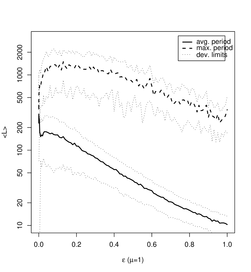
Figure 5: The period of the observed limit cycles, averaged over 100 trials, decreases roughly exponentially as the noise amplitude $\varepsilon$ increases (for $\mu=1$, $N=50$; note the semi-logarithmic scale.) The average period for 10 networks is plotted as a solid line, and the average of the maximum periods for these 10 networks is plotted as a thick dashed line, with $1\sigma$ deviation limits plotted as dotted lines.

Figure 6: The total number of different limit cycles observed increases as the noise amplitude $\varepsilon$ increases (for $N=50$, and for a maximal number of trials $=1000$, in linear and log-log plots). For $\varepsilon>10^{-3}$, the ensemble-average scaling is approximately as a power law, ${\cal N}_{\text{cycles}}\sim\varepsilon^{\alpha}$, with $\alpha\sim 1.0$, making it roughly a linear function as well.

3.1 Eligibility

Since we are interested in complex dynamical behaviour, a large fraction of neurons should participate non-trivially in the dynamical collective activity of the network – such a network is said to have a high degree of eligibility. A limit cycle $\alpha$ will have a maximally eligible time-averaged firing pattern $\bar{{\boldsymbol{x}}}^{\alpha}$, if $\bar{x}_{i}^{\alpha}=\frac{1}{2}$ for all neurons $i$. There will be minimal eligibility if $\bar{x}_{i}^{\alpha}\in\{0,1\}$ for all neurons $i$. The Shannon information (or entropy) has these properties, so we will adopt an entropy function as our measure of the eligibility of a given limit-cycle attractor $\alpha$:

$$e(\alpha)\equiv-\frac{1}{N}\sum_{i=1}^{N}\bar{x}_{i}^{\alpha}\ln\bar{x}_{i}^{\alpha}.$$ (9)

The mean eligibility ${\cal E}$, averaged over all ${\cal N}_{\text{trials}}$ trials, is

$${\cal E}\equiv\frac{1}{{\cal N}_{\text{trials}}}\sum_{\alpha=1}^{{\cal N}_{\text{trials}}}e(\alpha)\leq\frac{1}{2}\ln 2\equiv{\cal E}_{\text{max}}$$ (10)

for fixed network connectivity and fixed $\varepsilon$. Despite its utility, we do not have a rigorous dynamical motivation for quantifying eligibility by entropy. As discussed at the beginning of this section, the fraction of actively participating neurons decreases with growing $\varepsilon$; thus eligibility is decreasing as well (Figure 9). In other words, when the thresholds become grossly ‘out-of-tune’ with the mean membrane potential, the RSANN attractors become more trivial, with each neuron tending toward its own independent fixed point $x_{i}(t)=1$ or $x_{i}(t)=0$.

3.2 Diversity

We measure the accessibility of a given attractor by estimating the probability $P(\alpha)$ that a given attractor (first observed at trial $\alpha$) is observed during all ${\cal N}_{\text{trials}}$ trials, identified with its relative frequency of occurence

$$P(\alpha)\equiv\frac{{\cal N}(\alpha)}{{\cal N}_{\text{trials}}}\;,$$ (11)

where ${\cal N}(\alpha)$ is the number of observations of limit cycle $\alpha$. Note that if a given attractor is only observed once, then $P(\alpha)=1/{\cal N}_{\text{trials}}$, while if the same attractor is observed in every trial, then $P(\alpha)=1$.

Given that each different limit-cycle attractor is accessed by the network with probability $P(\alpha)$, we can define the diversity ${\cal D}$ as the attractor occupation entropy:

$${\cal D}=-\sum_{\alpha=1}^{{\cal N}_{\text{cycles}}}P(\alpha)\ln P(\alpha)\;\text{ , where}\quad\sum_{\alpha=1}^{{\cal N}_{\text{cycles}}}P(\alpha)=1$$ (12)

and ${{\cal N}_{\text{cycles}}}$ is the total number of different observed cycles. It is easily seen that a large ${\cal D}$ corresponds to the ability to occupy many different cyclic modes with nearly equal probability; the diversity will reach a maximum value of ${\cal D}_{\text{max}}=\ln{{\cal N}_{\text{trials}}}$ when $P(\alpha)=1/{{\cal N}_{\text{trials}}}$ for all limit cycles $\alpha$, i.e. if in each trial a different cycle is observed. A small value of ${\cal D}$ corresponds to a strong stability (or inflexibility) of the system – very few different cyclic modes are available. As can be seen from Figure 9 the diversity grows rapidly with increasing disorder amplitude $\varepsilon$, and with a relatively small disorder value of $\varepsilon=\varepsilon_{1}\sim 10^{-2}$, the diversity is already half of its maximal value. Since it takes into account the accessibility of all the detected cycles, this technique of quantifying diversity by an entropy function is considerably more robust and meaningful than simply counting the cycles.

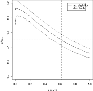
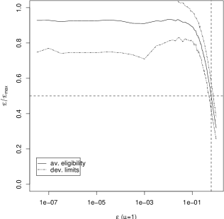
Figure 7: The mean eligibility ${\cal E}$ decreases with growing noise amplitude $\varepsilon$. We present two views for Figs. 8-10, one with a semi-logarithmic scale, so that both the small-$\varepsilon$ and large-$\varepsilon$ behavior can be inspected ($N=50$ for Figs. 8-10).

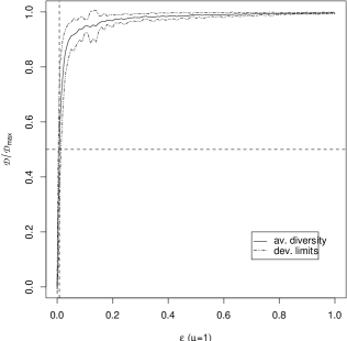
Figure 8: The diversity increases rapidly with growing noise amplitude $\varepsilon$ (note the log scale for $\varepsilon$ in one of these views).

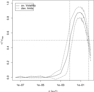
Figure 9: The volatility increases rapidly with growing noise amplitude due to the increasing diversity, as seen with both a linear and logarithmic scale in $\varepsilon$. It is large and nearly maximal within a rather broad range of noise amplitudes: $10^{-2}<\varepsilon<0.5$.

3.3 Volatility

Volatility is defined as the ability to access a large number of highly eligible limit cycles, or a ‘mixture’ of high eligibility and high diversity. Having defined both eligibility and diversity, we can now combine them to define volatility as an entropy-weighted entropy:

$${\cal V}=-\sum_{\alpha=1}^{{\cal N}_{\text{cycles}}}e(\alpha)P(\alpha)\ln P(\alpha)\;.$$ (13)

Since the volatility curve in Figure 9 is roughly the product of the eligibility and the diversity curve in Figures 9 and 9, there exists an intermediate regime $\varepsilon_{1}<\varepsilon<\varepsilon_{2}$ of high volatility. At $\varepsilon=\varepsilon_{1}\sim 10^{-2}$ the growing disorder amplitude causes a transformation to a condition of diversity, entailing many different limit cycles, whereas at $\varepsilon=\varepsilon_{2}\approx 0.5$ the disorder amplitude has become so large that most limit cycles become fixed points. We accordingly identify three different regimes for the RSANN with disorder:

1. Stable Regime: $\varepsilon<10^{-2}$

2. Volatile Regime: $10^{-2}\leq\varepsilon\leq 0.5$

3. Trivially Random Regime: $\varepsilon>0.5$.

3.4 Larger Ensemble study

Figure 10: For 300 networks of $N=50$ neurons, each with different connection strength matrices, we form histograms of the number of limit cycles found in each different network. Histograms for four different values of $\varepsilon$ are presented. Note the rebinned histogram in the inset of the $\varepsilon=0.0$ histogram.

The results obtained in Sections 3.1 - 3.3 were obtained from ten RSANNs with random weight matrices drawn from the uniform distribution $w_{ij}\in[-1,1]$. As can be seen from the standard deviation curves in figures 9- 9, which are in close proximity to the average curves, all networks exhibit the same qualitative behaviour. To further confirm this finding, we have tabulated in tables 1 & 2 and Figure 10 the statistics of the number of different limit cycles, their periods, and the diversity & volatility, for 300 networks with different connection strength matrices using 500 different disorder vectors ${\boldsymbol{\eta}}$ for each network. The $\varepsilon=0.0$ results in Table 1 and Figure 10 confirm Amari’s theoretical result (1974) and the empirical results of Clark, Kürten & Rafelski (1988), that random networks tend to possess only a small number of different cyclic modes. For larger $\varepsilon$, the ensemble-average number of cycles, the diversity and volatility are all much larger than for $\varepsilon=0$.

In particular, the results shown in Table 2 suggest that with increasing $\varepsilon$, the minimum period rapidly decreases, whereas the maximum period rapidly increases, with the average period staying roughly constant and closer to the minimum than the maximum. This suggests that at least a few limit cycles having long periods exist with non-normal thresholds, and that there are many more fixed points than long-period limit cycles when the thresholds are far from normal, than when the thresholds are close to normal.

	Number of different cycles (300 matrices)
$\varepsilon$	max. # of cycles	ave. # of cycles	ave. # of long cycles	diversity	volatility
0.0	6	2.11 $\pm$ 1.17	0.04 $\pm$ 0.19	0.06 $\pm$ 0.08	0.03 $\pm$ 0.04
0.1	176	45.58 $\pm$ 26.54	1.59 $\pm$ 2.12	0.33 $\pm$ 0.14	0.26 $\pm$ 0.10
0.2	422	179.98 $\pm$ 69.87	12.66 $\pm$ 12.89	0.70 $\pm$ 0.12	0.55 $\pm$ 0.12
0.4	500	461.34 $\pm$ 44.24	18.40 $\pm$ 19.89	0.98 $\pm$ 0.04	0.64 $\pm$ 0.14

Table 1: For 300 networks of $N=50$ neurons, each with a different matrix of connection strengths, we tabulate the statistics of the number of observed limit cycles (maximum number, average number of cycles, and average number of long cycles), as well as the average diversity and the average volatility. The results are given for 4 different values of threshold disorder $\varepsilon$.

	Average period length (300 matrices)
$\varepsilon$	ave. min. period	ave. max. period	ave. mean period
0.0	64.98	111.97	85.63
0.1	2.10	796.63	89.18
0.2	1.27	1233.89	146.66
0.4	1.02	1144.64	110.15

Table 2: For 300 networks of $N=50$ neurons, each a different matrix of connection strengths, we tabulate the averages of the statistics of the observed periods of the limit cycles for each network (minimum period, maximum period, mean period), for four different values of the threshold disorder $\varepsilon$.

3.5 Stability and attractor basins of observed cycles

We have shown in Sections 3.1 - 3.4 that when we change the threshold parameters of a network sufficiently far from their default values, then we get new, non-trivial behavior for nearly each parameter realization. Since the level of threshold disorder which is needed to obtain new and complex behavior is not too high, the ensemble of networks can exhibit diverse and complex behavior with only slight changes in the network parameters.

Figure 11: The number of repeatedly observed limit cycles with a fixed set of connection strengths and thresholds but different initial conditions ${\boldsymbol{x}}(0)$ is relatively stable with $N_{\text{cycles}}^{\text{fixed}}\sim 2\pm 1$. (for $N=50$ and $\mu=1$; with 100 random initial conditions, averaged over several threshold realizations; the solid curve is a smoothed average curve; the dotted curves are smoothed $1\sigma$ error curves).

Figure 12: The attractor occupation entropy (Eq. 12) of the small number of observed cycles (compare Fig. 12) allows us to estimate the relative sizes of the basins of attraction. Since the entropy reaches only half of its maximum, some cycles dominate over the others. The solid curve is a smoothed average curve; the dashed curves are smoothed $1\sigma$ error curves.

In order to demonstrate that this diversity originates only from ensemble diversity and is not intrinsic to the specific network realizations, we must show that each specific network of the ensemble possesses only a limited set of limit cycles. For this reason we counted the number of different observed cycles ${\cal N}_{\text{cycles}}^{\text{fixed}}(w_{ij},{\boldsymbol{\eta}}(\varepsilon))$ of each network $(w_{ij},{\boldsymbol{\eta}}(\varepsilon))$ in the ensemble starting with 100 randomly-chosen initial activity patterns ${\boldsymbol{x}}(0)$. Then we performed the ensemble average

$${\cal N}_{\text{cycles}}^{\text{fixed}}(\varepsilon)=\langle{\cal N}_{\text{cycles}}^{\text{fixed}}(w_{ij},{\boldsymbol{\eta}}(\varepsilon))\rangle_{{\boldsymbol{\eta}}(\varepsilon)}\,.$$ (14)

As can be seen from Figure 12, the number of different observed cycles is rather small, and does not depend upon the disorder amplitude $\varepsilon$. Of course, the actual size of the repertoire does depend on the instantiation of ${\boldsymbol{\eta}}(\varepsilon)$, as evidenced by the deviations (indicated by dashed curves), but the degree of variation in ${\cal N}_{\text{cycles}}^{\text{fixed}}(\varepsilon)$ in no way matches the substantial secular increase of ${\cal N}_{\text{cycles}}^{\text{fixed}}(\varepsilon)$ observed in Figure 6.

Using a similar diversity measure like in Equation 12, but now using the occurence probabilities of observed cycles with fixed network parameters, it is possible to estimate the relative sizes of the basins of attraction of these cycles. The diversity becomes maximal when all cycles are observed with equal probability, corresponding to basins of attractions of equal size. As can be seen from Figure 12, the diversity reaches only the half of its maximum, indicating basins of attraction of different sizes. The figure suggests that $-\langle\ln P\rangle\sim\frac{1}{2}$, implying that $\langle P\rangle\sim 0.6$. In other words, for fixed thresholds, as we vary the initial firing vector, we observe the same cycle in greater than $\sim 60\%$ of the trials; as evident in Figure 12, there is little dependence in the fixed-threshold cycle-diversity upon the frozen-disorder amplitude $\varepsilon$.

3.6 Distribution of Limit-Cycle Periods and their Dependence upon Network Size

For the choice of threshold and connectivity parameters made here, the average cycle length $\langle L\rangle$ grows exponentially with the network size $N$ (see Fig. 14). This exponential scaling of the cycle length puts it in the ‘chaotic’ regime of Kürten’s (1988) classification of dynamical phases, where the motion shows high sensitivity to initial conditions. Kürten also found a ‘frozen’ regime where the limit-cycle period scales as a power law in $N$, and where there is little sensitivity of the attracting limit cycle upon initial conditions. When $\varepsilon=0.02$, which is in the volatile region, a broad, non-gaussian distribution of cycle lengths is found (see Fig. 14). Furthermore, since the cycle-length distribution shown in Fig. 14 does not exhibit peaks at regularly spaced intervals, the possibility that we have employed an errant limit-cycle comparison algorithm is unlikely. This distribution of cycle-lengths for RSANNs differs significantly from the $\exp(-L^{2}/\tau^{2})/L$ distribution of cycle-lengths predicted for Kauffman’s Boolean nets by Bastolla and Parisi (1997). This difference in distributions implies that there may be some significant differences between these two types of nets.

Figure 13: Mean cycle length $\langle L\rangle$, averaged over 20 weight matrices with normal thresholds and $\varepsilon=0.1$, grows exponentially with network size $N$. In Figure 14, we observe that the distribution of limit-cycle periods for fixed $N$ has a broad range of periods ranging from $L=1$ to roughly $2\langle L\rangle$. Therefore, using standard error bars on the values of $\langle L\rangle$ in the above plot would not be very informative.

Figure 14: Distribution of different limit-cycle periods observed in the volatile regime ($N=50$, $\varepsilon=0.02$). We overlay a fit to the distribution predicted by Bastolla & Parisi (1997, 1997b) for Kauffman nets.

3.7 Dependence of Attractor Count on Observation-Period Length

In Figure 6, we showed that the number of different attractors observed, ${\cal N}_{\text{cycles}}$, is a significant fraction of the total number of trials ${\cal N}_{\text{trials}}$ when $\varepsilon>0.1$. For disorder between $\varepsilon=10^{-2}$ and $\varepsilon=0.1$, the number of cycles observed is much larger than one (see Figure 9.b), but less than the total number of trials. In the stable regime ($\varepsilon<10^{-2}$),  ${\cal N}_{\text{cycles}}$ is quite small and largely independent of ${\cal N}_{\text{trials}}$. These three results are complementary: the first result (at high $\varepsilon$) implying a nearly inexhaustible source of different limit-cycle attractors accompanied by a steady decrease of eligibility with increasing $\varepsilon$; the second result (at moderate $\varepsilon$) implying a large, but limited repertoire of limit cycles of high eligibility; and the third result (at very low $\varepsilon$) implying that we can exhaustively access a small group of high-eligibility limit-cycle attractors with a high degree of robustness.

In the stable regime, ${\cal N}_{\text{cycles}}$ is often greater than $1$ (though small), which means that the stable phase cannot be used to access a particular attractor upon demand, but we can demand reliable access to one of a small number of different attractors. Frequently, however, there is a single dominant attractor, as indicated by the low entropy seen in Fig. 12. We conclude that, in practice, for a given set of network parameters or external inputs to the network, but starting with different initial conditions, the network will converge to the same attractor most of the time.

4 Discussion

4.1 Ensemble-scanner, Multistability, ‘Creativity/Madness’, and Control Algorithms

In the ‘noisy’ runs at $\varepsilon>0$, epitomized by Fig. 1, we are actually sampling a significant fraction of an entire ensemble of closely-related networks over the course of time, as the noise or disorder or an external input slowly varies. Based upon the results for our RSANN model, quenched noise (disorder) can give a dynamical system access to a whole ensemble of different behaviors at different times during the lifetime of the dynamical system. In other words, slowly-varying threshold noise or disorder or external input can act as a ‘scanner’ for a host of dynamic modes.

The posed existence (Skarda & Freeman (1987), Yao & Freeman (1990), Freeman et al. (1997)) of a chaotic ground-state attractor for the olfactory system and the existence of ‘multistable’ limit-cycle excited-state attractor lobes provides a striking exemplification of our volatility concept, and potentially an in vivo demonstration of this phenomenon.

The RSANN networks studied here have a small repertoire of behaviors when there is no noise or disorder in the thresholds ($\varepsilon=0$); hence, there is little multistability. The size of the repertoire becomes tremendously large (as does the extent of multistability) for ‘small’ changes in the threshold parameters ($\varepsilon>10^{-2}$). One is therefore tempted to call this behavior ‘chaotic’ with respect to the parameter changes, since it has one of the hallmarks of chaos (sensitive dependence upon small changes of the parameters). However, for smaller changes in the threshold parameters ($0<\varepsilon<10^{-3}$), the repertoire of $\varepsilon=0$ behaviors is ‘stable’ – no new cycles are observed. For the purpose of discussion , we refer to this delimited sensitivity to parameter changes, as ‘quasi-chaos’ or ‘quasi-multistability’. Additionally, the stability is augmented by the fact that very frequently, the repertoire of a network in the stable regime is dominated by a single cycle (for fixed connections and fixed disorder), a phenomenon known as ‘canalization’ (Kauffman (1993)). Hence, for the sake of argument, we will also assume that in the stable regime only one cycle is accessible. By taking advantage of the quasi-chaotic/quasi-multistable threshold parameters (noting that the connection strength parameters are probably also quasi-chaotic), we can access a large number of different RSANN attractors, each with a small neighborhood of stability in threshold-parameter space. With a suitable feedback algorithm, one might be able to control this quasi-chaos (cf. Ott, Grebogi & Yorke (1990)) and access and stabilize a given attractor upon demand. Due to the proximity of other limit cycles just beyond the local neighborhood of stability of the given attractor, novel attractors are always within a stone’s throw of the given attractor, while maintaining a respectable distance so as not to be destabilizing. Such an approach to controlled creativity has been developed into the adaptive resonance formalism (Carpenter & Grossberg (1987)).

The volatile regime within $\varepsilon=0.001-0.5$ can be subdivided into two sub-regimes. The lower end of the range, $\varepsilon=0.001-0.1$, which corresponds to the upward-sloping part of the volatility curve in Figure 9.b, could suggestively be named the ‘creative’ regime, wherein new cycles are observed with some rarity, so as to provide truly new behavioral modes for the RSANN. These new cycles can be taken together with the more commonly-observed cycles in the net’s repertoire, perhaps to produce new and ‘interesting’ sequences of behavior (if these cyclic modes can be logically sequenced). The upper end of the range, $\varepsilon=0.1-0.5$, might be regarded as the ‘overly-creative’ or ‘slightly-mad’ regime of the RSANN. New, rather complex modes are being found with almost every trial, which could overwhelm the ‘bookkeeping’ resources necessary for the RSANN to implement or utilize the new mode to its full potential. Clearly, this abstract and simple RSANN model is insufficent to be a true neurobiological model of creativity/madness, but it could be a good starting point for a more detailed model.

4.2 Generalization to other Complex Systems

It may well be a common feature of a broad class of complex, non-linear systems without adaptability or noise that the diversity of non-trivial behaviors is limited. We have confirmed the lack of diverse behavior for a non-linear system with truly simple elements (McCullough-Pitts neurons); we have also seen similar non-volatile behavior for a slightly more general, discretized integrate-and-fire neuron model. This canalization result may be generalizable to other complex systems of either simple or complex units. Indeed, one of the first observations of canalization was in Kauffman’s Boolean immunological networks, which have some significant differences from RSANNs. The canalization property might have been more difficult to generalize if we had started with more complex units like Hodgkin-Huxley neurons. Furthermore, it is plausible that the introduction of a moderate amount of noise or disorder will generally increase the diversity of complex behaviors, as we have seen in RSANNs.

Our volatility-producing model might be applicable in more abstract situations. One might imagine that the states of our simple Boolean neuron reflect in some manner the ‘on or off’ state of complex subunits of a modular system. Such modular complex systems could be probed to determine whether dynamical diversity can or cannot be enhanced by small changes in network parameters. Examples might include:

1. A random neural network composed of subnetworks;

2. A network of complex, real neurons;

3. The brain of an organism with its different subsystems;

4. The geoeconomic or political structure of a large country composed of smaller states, regions, or cities; and

5. The ecological network of the world composed of different regions or of different subcommunities of animals or plants.

In models with subunits that are composed of many sub-subunits, the stability or canalizing ability of the system itself may be significantly enhanced either by a law-of-large-numbers decrease in the noise/disorder susceptibility of an individual subunit, or by self-stabilizing internal feedback loops which may be present by design within the subunits.

4.3 Conclusions & Prospects

Based on combinatorics and statistical arguments, one expects to find many limit cycles in a random synchronous asymmetric neural network (RSANN). Experience has shown otherwise. After much of this paper was completed, we found an analytical argument by Amari (1974, 1989) to the effect that RSANNs have only one attractor, in the thermodynamic limit of a large number of neurons, thus explaining our $\varepsilon=0$ results.

The main objective of our study has been to construct a volatile neural network which exhibits a large set of easily-accessible highly-eligible limit-cycle attractors, as has been achieved already in a non-neural system (Poon & Grebogi (1995)). First, we have demonstrated that in the absence of noise and in the absence of random, long-term imposition of threshold disorder, a random asymmetric neural network can reach only a small number of different limit-cycle attractors. Second, by imposing and freezing neuronal threshold disorder within a well-defined range ($\varepsilon_{1}<\varepsilon<\varepsilon_{2}$), we show that RSANNs can access a diversity of highly-eligible limit-cycle attractors. RSANNs exhibit a phase transformation from a small number of distinct limit-cycle attractors to a large number at a disorder amplitude of $\varepsilon=\varepsilon_{1}\sim 10^{-2}$. Likewise, RSANNs exhibit an eligibility phase transformation at a threshold disorder amplitude of $\varepsilon=\varepsilon_{2}\sim 0.5$.

Potentially, Amari’s argument can be extended to gain an understanding of how slight changes of threshold parameters beyond some minimal level can substantially increase the diversity of accessible cyclic modes. This extension is beyond the scope of the current work. Another very interesting question is how the diversity and volatility curves scale with the size of the network.

While the addition of threshold disorder seems to be a trivial mechanism for enhancing the volatility or diversity by constantly changing the parameters of the RSANN, we believe that since some biological systems (Neiman et al. (1999)) may use threshold, synapse and/or externally-generated noise or disorder to enhance their abilities, we have discovered a simple feature which could have some importance in modeling biological systems. We fully expect that other volatility-enhancing mechanisms are available beyond the particular one proposed here.

In summary, our key result is that a random neural network can be driven easily from one to another stable recurrent mode. While such behavior can be always accomplished by radical modifications of some of the network properties, the interesting result we have here presented is that plausibly small (e.g., RMS in the neighborhood of 0.1-1%) and random changes imposed simultaneously upon all of the neural threshold parameters suffices to access new dynamical behavior. Indeed, due to the combinatorics of changing many parameters simultaneously, an immense number of interesting modes become available to the system. We are aware that this does not yet create a network that can self-sequence a series of modes, though some authors have already made considerable progress in this direction (e.g. Daucé and Quoy (2000), Tani (1998)). The development of autonomous control algorithms that provide access to mode sequences is a natural but challenging objective that can potentially lead to a deeper understanding of information processing in recurrent neural networks.

Acknowledgements

H. Bohr would like to acknowledge the hospitality of P. Carruthers (now deceased), J. Rafelski, and the U. Arizona Department of Physics during several visits when much of this work was carried out. During his graduate studies, P. McGuire was partially supported by an NSF/U.S. Department of Education/State of Arizona doctoral fellowship. J.W. Clark acknowledges research support from the U.S. National Science Foundation under Grant No. PHY-9900713. McGuire, Bohr and Clark were participants in the Research Year on the “The Sciences of Complexity: From Mathematics to Technology to a Sustainable World” at the Center for Interdisciplinary Studies (ZiF) at the University of Bielefeld, in Germany. We all thank many individuals who have provided different perspectives to our work, including the following: G. Sonnenberg, D. Harley, Z. Hasan, H. Ritter, R. Vilela-Mendes, and G. Littlewort.

References

- [1] S. Amari, “A Method of Statistical Neurodynamics,” Kybernetik, 14 (1974) 201.
- [2] S. Amari, “Mathematical Foundations of Neurocomputing,” Proceedings of the IEEE, 78 (1990) 1443; University of Tokyo Mathematical Engineering Technical Report 89-06.
- [3] U. Bastolla and G. Parisi, “Attractors in Fully Asymmetric Neural Networks,” J. Phys. A: Math. Gen. 30 (1997) 5613.
- [4] U. Bastolla and G. Parisi, “Attraction Basins in Discretized Maps,” J. Phys. A: Math. Gen., 30 (1997b) 3757.
- [5] P. C. Bressloff and J. G. Taylor, “Random Iterative Networks,” Phys. Rev. A41 (1990) 1126.
- [6] J. Buhmann and K. Schulten, “Influence of Noise on the Function of a ‘Physiological’ Neural Network,” Biol. Cybern. 56 (1987) 313.
- [7] G.A. Carpenter and S. Grossberg, “ART 2: Self-organization of Stable Category Recognition Codes for Analog Input Patterns,” Applied Optics 26 (1987) 4919.
- [8] C.C. Chow and J.A. White, “Spontaneous Action Potentials due to Channel Fluctuations,” Biophysical J. 71 (1996) 3013.
- [9] J.W. Clark, “Statistical Mechanics of Neural Networks,” Phys. Rep. 158 (1988) 9.
- [10] J.W. Clark, “Long-term Behavior of Neural Networks,” Relaxation Complex Systems and Related Topics, eds. I. Campbell and C. Giovannella (Plenum: New York, 1990) 205.
- [11] J.W. Clark, “Neural Network Modelling,” Phys. Med. Biol. 36 (1991) 1259.
- [12] J.W. Clark, K.E. Kürten and J. Rafelski, “Access and Stability of Cyclic Modes in Quasirandom Networks of Threshold Neurons Obeying a Determinisitic Synchronous Dynamics,” Computer Simulation in Brain Science, edited by R.M.J Cotterill (Cambridge Univ. Press:Cambridge,1988) 316.
- [13] J.W. Clark, J. Rafelski and J.V. Winston, “Brain Without Mind: Computer Simulation of Neural Networks with Modifiable Neuronal Interactions,” Phys. Rep. 123 (1985) 215.
- [14] E. Daucé and M. Quoy, “Resonant Spatio-temporal Learning in Sparse Random Recurrent Networks,” submitted to Biol. Cybernetics (2000).
- [15] W.J. Freeman, H.J. Chang, B.C. Burke, P.A. Rose, and J. Badler, “Taming Chaos: Stabilization of Aperiodic Attractors by Noise,” IEEE Trans. on Circuits and Systems, 44 (1997) 989.
- [16] C.M. Gray & W. Singer, “Stimulus-specific Neuronal Oscillations in Orientation Columns of a Cat Visual Cortex” Proceedings of the National Acadamey of Sciences, USA 86 (1989) 1698.
- [17] Z. Hasan, “Biomechanical Complexity and the Control of Movement,” Lectures in the Sciences of Complexity, edited by D.L. Stein (Santa Fe Institute Studies in the Sciences of Complexity, Addison-Wesley) (1989) 841.
- [18] J.J. Hopfield, “Neural Networks and Physical Systems with Emergent Collective Computational Abilities,” Proc. Natl. Acad. Sci. USA 79 (1982) 2554.
- [19] Stuart A. Kauffman, The Origins of Order: Self-Organization and Selection in Evolution, Oxford University Press (1993).
- [20] K.E. Kürten, “Critical Phenomena in Model Neural Networks,” Phys. Lett. A129 (1988) 157.
- [21] H. Lecar and R. Nossal, “Theory of Threshold Fluctuations in Nerves. I. Relations between Electrical Noise and Fluctuations in Axon Firing,” Biophysical J. 11 (1971) 1048.
- [22] H. Lecar and R. Nossal, “Theory of Threshold Fluctuations in Nerves. II. Analysis of Various Sources of Membrane Noise,” Biophysical J. 11 (1971) 1068.
- [23] W.A. Little, “The Existence of Persistent States in the Brain,” Math. Biosci. 19 (1974) 101.
- [24] G.C. Littlewort, J.W. Clark and J. Rafelski, “Transition to Cycling in Neural Networks,” Computer Simulation in Brain Science, edited by R.M.J Cotterill (Cambridge Univ. Press:Cambridge,1988), 345
- [25] Z.F. Mainen and T.J. Sejnowski, “Reliability of Spike Timing in Neocortical Neurons,” Science 268 (1995) 1503.
- [26] E. Marder and S.L. Hooper, “Neurotransmitter Modulation of the Stomatogastric Ganglion of Decapod Crustaceans,” Model Neural Networks and Behavior, editted by A.I. Selverston (Plenum Press: New York,1985), 319.
- [27] P.C. McGuire, G.C. Littlewort and J.Rafelski, “Brainwashing Random Asymmetric ‘Neural’ Networks,” Phys. Lett. A160 (1991) 255.
- [28] P.C. McGuire, G.C. Littlewort, C. Pershing and J. Rafelski, “Training Random Asymmetric ‘Neural’ Networks Towards Chaos – A Progress Report,” Proceedings of the Workshop on Complex Dynamics in Neural Networks,edited by J.G Taylor, E.R. Caianiello, R.M.J. Cotterill and J.W. Clark ( Springer-Verlag, London, 1992) pp. 90-102.
- [29] J.D. Murray, Mathematical Biology, Springer-Verlag (1989), pp. 161-166.
- [30] A. Neiman, X. Pei, D. Russell, W. Wojtenek, L. Wilkens, F. Moss, H. Braun, M. Huber and K. Voight, “Synchronization of the Electrosensitive Noisy Cells in the Paddlefish,” Phys. Rev. Lett. 82 (1999) 660.
- [31] E. Ott, C. Grebogi and J.A. Yorke, “Controlling Chaos,” Phys. Rev. Lett. 64 (1990) 1196.
- [32] X. Pei, L.A. Wilkens and F. Moss, “Noise-mediated Spike Timing Precision from Aperiodic Stimuli in an Array of Hodgkin-Huxley-type Neurons,” Phys. Rev. Lett. 77 (1996) 4679.
- [33] L. Poon and C. Grebogi, “Controlling Complexity,” Phys. Rev. Lett. 75 (1995) 4023-4026.
- [34] R.H. Rand, A.H. Cohen and P.J. Holmes, “Systems of Coupled Oscillators as Models of Central Pattern Generators,” Neural Control of Rhythmic Movements in Vertebrates, Eds. A.H. Cohen, S. Rossignol, and S. Grillner (John Wiley: New York, 1988), 333.
- [35] M. Schreckenberg, “Attractors in the Fully Asymmetric SK-model,” Z. Phys. B - Condensed Matter 86, (1992) 453.
- [36] G. L. Shaw and R. Vasudevan, “Persistent States of Neural Networks and the Random Nature of Synaptic Transmission,” Math. Biosci., 21 (1974) 207.
- [37] C.A. Skarda and W.J. Freeman, “How Brains Make Chaos in Order to Make Sense of the World,” Behavioral and Brain Sciences, 10 (1987) 161.
- [38] J. Tani, “An Interpretation of the ‘Self’ from the Dynamical Systems Perspective: a Constructivist Approach”, J. Consciousness Studies 5 (1998) 516.
- [39] J. G. Taylor, “Spontaneous Behaviour in Neural Networks,” J. Theor. Biol., 36 (1972) 513.
- [40] Y. Yao and W.J. Freeman, “Model of Biological Pattern Recognition with Spatially Chaotic Dynamics,” Neural Networks, 3 (1990) 153.
- [41] A. Zador, “Impact of Synaptic Unreliability on the Information Transmitted by Spiking Neurons,” J. Neurophysiol. 79 (1997) 1219.