Low temperature value of the upper critical field $H_{c2}(0)$ of isotropic single band metals

Abstract

The strong coupling Schossmann-Schachinger theory for the upper critical field is considered methodically from the user point of view. We check the accuracy of approximate formulas for the upper critical field. In particular, we explain in detail as a recently proposed convenient expression (Shulga et al. cond-mat/0103154) can be justified. The connection of $H_{c2}(0)$ with the critical temperature $T_{c}$ is considered and the similarity with the Allen-Dynes $T_{c}$-formula is shown explicitly.

I Introduction

The standard isotropic single band (ISB) Eliashberg model [1] is the most developed part of the modern theory of superconductivity. It describes quantitatively the renormalization of the physical properties of metals due to the electron-phonon interaction. The input material parameters are the density of states at $E_{F}$, $N(0)$, the bare Fermi velocity $v_{F}$, the impurity scattering rate $\gamma_{imp}$, the paramagnetic impurity scattering rate $\gamma_{m}$, the Coulomb pseudopotential $\mu^{*}(\approx 0.1)$, and the electron-phonon spectral (Eliashberg) function $\alpha^{2}F(\Omega)$. Thereby the validity of the Born approximation is assumed, i.e. the system is far from the onset of localization.

These days the material parameters $N(0)$, the averaged Fermi velocity, and the spectral function become available from microscopic calculations just very soon after the discovery of a new superconducting compound. The standard procedures of analysis of many physical properties of metals include these results as input parameters. For example, the density of states $N(0)$ is important for the description of the specific heat data. Similarly, the calculated plasma frequency is used for the interpretation of the optical and transport properties. As a rule, the forthcoming optical measurements do confirm its value later on. At the same time, the upper critical field $H_{c2}(0)$, the fundamental quantity of a type-II superconductors is usually analyzed by experimentalists in the framework of the phenomenological Ginzburg-Landau (GL) theory which states $H_{c2}(0)=\Phi_{0}/2\pi\xi^{2}$. Here $\Phi_{0}$ is the flux quantum and $\xi$ is the GL-coherence length, the material parameter of the GL theory.

Within the Eliashberg ISB model $H_{c2}(T)$ can be computed using the Schossmann-Schachinger self-consistent theory [2]. This theory treats $H_{c2}(T)$ as the field dependence of the critical temperature $T_{c}(H)$. At $H=0$ the linear $H_{c2}(T)$-problem is reduced to the equations for $T_{c}$. From a numerical point of view the eigenvalue problems for $T_{c}$ and $H_{c2}(T)$ are identical and can be computed by the same code. In practice, however, the linearized equations for $T_{c}$ are frequently not exploited even by teams who perform tedious numerical band structure or Eliashberg-theory calculations. Instead the well-known phenomenological Allen-Dynes expression for $T_{c}$ is widely used. In our opinion a similar approach could be applied also to $H_{c2}(0)$ calculating it from a simple formula.

Here, for the sake of clarity and simplicity the Pauli limiting, unimportant in many cases of practical interest, is ignored. In the present paper we examine five simple expressions for $H_{c2}(0)$ by comparison with the numerical solutions of Eqs. 1-5. One of these formulas valid in the clean limit is presented in the present work for the first time. It is shown that at least three formulas fit reasonably well the numerical values of $H_{c2}(0)$ in a wide range of coupling strengths $\lambda$. The deviations do not exceed 12%. Extensions to cases of arbitrary impurity content are considered as well. An application example of the approximate phenomenological formula is provided.

II General equations and approximate semi-analytical formulas

To take into account fully retardation and strong coupling effects in calculating $H_{c2}$, we have solved numerically the linearized equations proposed in Ref.[2]

$$\tilde{\omega}(n) = \omega_{n}+\frac{\gamma_{imp}{\rm sgn}\omega_{n}}{2}+\pi T\sum_{m}\lambda(m-n)\mbox{sgn}\omega_{m},$$ (1)

$$\tilde{\Delta}(n) = \pi T\sum_{m}\frac{[\lambda(m-n)-\mu^{*}]\tilde{\Delta}(m)}{\chi^{-1}(m)-\gamma_{imp}/2},$$ (2)

$$\chi(n) = \frac{2}{\sqrt{\beta}}\int_{0}^{\infty}dqe^{-q^{2}}{\rm atan}\left[\frac{q\sqrt{\beta}}{|\tilde{\omega}(n)|}\right],$$ (3)

$$\beta = \hbar eH_{c2}v_{F}^{2}/2c,$$ (4)

$$\lambda(n) = \int_{0}^{\infty}d\omega\omega\alpha^{2}F(\omega)/[\omega^{2}+(2\pi Tn)^{2}].$$ (5)

Here $\omega_{n}$=$\pi T(2n+1)$ are the Matsubara frequencies, $e$ and $\tilde{\Delta}(n)$ denote the electron charge and the superconducting order parameter. $\hbar$ and $c$ are the Plank’s constant and the speed of light.

From the numerical point of view the equations of the Werthamer-Helfand-Hohenberg (WHH) [3] and the Schossmann-Schachinger theory have the same order of complexity. At the same time the WHH equations allow full analytical solutions, both in the clean and dirty limits. In particular, the clean limit WHH orbital upper critical field for the ISB model reads

$$H_{c2}^{{\rm WHH}}(0)=\frac{k_{B}^{2}T_{c}^{2}\pi^{2}ce^{2-\gamma}}{2\hbar ev_{F}^{2}},$$ (6)

where $k_{B}$ and $\gamma$=0.577 denote the Boltzmann’s and the Euler’s constants. In practical units this formula can be rewritten as

$$H_{c2}^{{\rm WHH}}(0)[{\rm Tesla}]=\frac{0.0231T_{c}^{2}[{\rm K}]}{v_{F}^{2}[{\rm 10^{7}cm/s}]}\approx\frac{0.02T_{c}^{2}[{\rm K}]}{v_{F}^{2}[{\rm 10^{7}cm/s}]}.$$ (7)

Within the BCS theory, where 2$\Delta\equiv 3.53T_{c}$, the formula

$$H_{c2}^{Sung}(0)=\frac{13.3c\Delta_{0}^{2}}{2e\hbar v_{F}^{2}},$$ (8)

is identical to the basic Eq. (6). It was used by Sung [4] for an estimation of $v_{F}$ in Nb.

McMillan and Werthamer [5] were the first who introduced the first order strong coupling corrections ($Z(0)=1+\lambda$)

$$H_{c2}^{{\rm McM-WHH}}(T)=H_{c2}^{{\rm WHH}}(T)(1+\lambda)^{2},$$ (9)

$$H_{c2}^{{\rm McM-WHH}}(0)=\frac{k_{B}^{2}T_{c}^{2}\pi^{2}ce^{2-\gamma}}{2\hbar e[v_{F}/(1+\lambda)]^{2}}=\frac{k_{B}^{2}T_{c}^{2}\pi^{2}ce^{2-\gamma}}{2\hbar e{v_{F}^{*}}^{2}}.$$ (10)

They conclude, that “this produces a substantial overall increase in $H_{c2}$ from that which would be obtained using the bare band Fermi velocity, but being relatively temperature-independent the shift cancels out of $h(t)$.” These days Eq. (10) is often regarded as a BCS formula since the “bare” Fermi velocity has to be replaced by the “dressed” Fermi velocity $v_{F}^{*}=v_{F}/(1+\lambda)$ in Eq. 6. Similarly, the renormalized form of Sung’s formula (8) reads

$$H_{c2}^{McMS}(0)=\frac{13.3c\Delta_{0}^{2}}{2e\hbar{v_{F}^{*}}^{2}}.$$ (11)

For the sake of completeness, we note that in the presence of magnetic pair-breaking the considered renormalization of $v_{F}$ is different [6].

Since there are no analytical solution of Eqs. (1-5), approximate expressions should be used to estimate $H_{c2}(0)$. The parameters in such formulas are determined by the fit of numerical data. The first expression [1] reads

$$H^{A}_{c2}(0)=\frac{T_{c}^{2}(1+\lambda)^{2}\pi^{2}ce^{2-\gamma}}{2\hbar ev_{F}^{2}}\left[1+1.44\left(\frac{T_{c}}{\omega_{\ln}}\right)\right],$$ (12)

where $\omega_{\ln}$ is the characteristic phonon frequency introduced by Kirzhnits et al. [7] and used later on in Ref. [13] by Allen and Dynes. A similar $H_{c2}(0)$ expression was proposed by Masharov [8] who obtained however different values for the numerical coefficients.

Our factorable formula, first presented here,

$$H^{C}_{c2}(0)\approx\frac{k_{B}^{2}T_{c}^{2}\pi^{2}ce^{2-\gamma}(1+\lambda)^{2.2}}{2\hbar e{v_{F}}^{2}},$$ (13)

is suitable for applications together with other factorable expressions. In practical units it reads

$$H^{C}_{c2}(0){\rm[Tesla]}\approx\frac{0.0231T_{c}^{2}[{\rm K}](1+\lambda)^{2.2}}{v_{F}^{2}[{\rm 10^{7}cm/s}]}.$$ (14)

Note that the choice of the coefficients in Eq. (14) is not unique. For example, the following expression

$$H^{B}_{c2}(0){\rm[Tesla]}\approx\frac{0.02T_{c}^{2}[{\rm K}](1+\lambda)^{2.4}}{v_{F}^{2}[{\rm 10^{7}cm/s}]},$$ (15)

demonstrates even better agreement with the numerical data. Eq. 15 is especially designed for the Q-check [9] in the spirit of the Langmann’s BCS Eq. 24 in Ref.[10].

III Results and Discussion

To check the accuracy of Eqs. (10-15), we solved the Eq. (1-5) employing an Einstein spectral function with various coupling constants $\lambda=0.7-2.9$ and standard values for the Coulomb pseudopotential $\mu^{*}$. Then the $H_{c2}(0)$-values from the approximate formulas (10-15) were normalized by the ”exact” numerical values. The result is shown in Fig. 1. If the symbol occurs below the unity line, the corresponding approximate expression underestimates $H_{c2}(0)$ and vice versa. The phenomenological formulas Eqs. (12-15) fit well the numerical data. The deviations from unity do not exceed 12% in a wide range of coupling strengths. The formulas Eqs. (10-11) being identical within BCS theory deviates differently and exhibit relatively lower accuracy.

A detailed discussion and collections of the BCS upper critical field formulas are given for instance in Ref. [11]. Here we discuss only the structure of weak coupling formulas Eqs. (10-11) with respect to the general Bergman-Rainer [14] ansatz

$$H_{c2}(0)=H_{c2}^{BCS}(0)f(\alpha^{2}F(\Omega),\mu^{*},T_{c}).$$ (16)

For the reason of dimensionality $H_{c2}^{BCS}(0)$ is proportional to the square of some typical energy. It could be $T_{c}$, the gap $\Delta_{0}$, the Debye energy $\omega_{D}$, or the average phonon frequency $\omega_{ln}$, and there is a total equivalence between them within the BCS theory due to its universal character. Within the Eliashberg theory the situation is different. Here Eq. (10) is more preferable than the renormalized Sung’s formula (11) (see Fig. 1). In fact, at given $\lambda$ the $H_{c2}^{McM-WHH}(0)$ points accumulate at nearly the same position for different values of $\mu^{*}$ in comparison with the $H_{c2}^{McMS}(0)$ data which spread out. This accumulation is a clear advantage of the basic Eq. (10). A similar choice in favor of Eq. (10) was made by Carbotte [1] without comments. We believe that the weak sensitivity of the ratio $H_{c2}(0)/T_{c}^{2}$ to details of $\alpha^{2}F(\omega)$ and the actual value of $\mu^{*}$ is due to the fact that $H_{c2}(0)$ and $T_{c}$ are the solution of the same linearized system of Eqs. (1-5) [12].

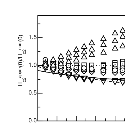
FIG. 1.: The upper critical field, normalized on the corresponding “exact” Schossmann-Schachinger numerical values, vs. coupling constant $\lambda$. Approximate basic WHH formula ($\bigtriangledown$, Eq. 10),renormalized Sung formula ($\bigtriangleup$, Eq. 11), Carbotte formula ($\Diamond$, Eq. 12), and our formulas ($\bigcirc$, Eq. 15 and $\Box$, Eq. 14) were indicated. The fitted functions $(1+\lambda)^{-0.231}$ and $0.02(1+\lambda)^{-0.4}/0.0231$ were shown by solid and dash-dotted lines. Identical symbols for the same $\lambda$ correspond to different standard values of the Coulomb pseudopotential $mu^{*}$=0.06, 0.1, and 0.14, respectively.

In Sec.  II various $H_{c2}(0)$ formulas are presented in different styles. The first group consists of “textbook-like” expressions(6,10,12,13) which contain explicitly fundamental physical and mathematical constants. Eqs. 7,14,15 written in practical units are preferred by insiders working in the field. Sung’s formulas (8,11) occupy an intermediate position. In our opinion the complete “textbook-like” presentation is necessary when a formula is derived for the first time from a general theory without simplifying additional assumptions. Otherwise, all styles are equivalent. In the present context a proof means a comparison of values given by a formula and a related computer code.

In view of a reasonable accuracy the question might arise: “Should we truncate higher digits in the prefactor $B_{1}=0.0231$ of Eq. 7 to $B_{2}=0.02$ before substitution into Eq. 16 or not?” because the Fermi velocity is not constant across the Fermi surface, and it is usually known with some uncertainty. The alternative possibilities led to Eqs. (13,14) and Eq. (15).

The Carbotte formula (12) also derived from Eqs. (1-5) through a series of simplifying assumptions, includes second order strong coupling corrections in terms of the small parameter $T_{c}/\omega_{ln}$. The leading linear term 1.44$T_{c}/\omega_{\ln}$ is introduced on a pure phenomenologically basis to get the best fit of numerical data (see remark below Eq. (7.15) in Ref. [1]). The Carbotte formula contains the additional parameter $T_{c}/\omega_{\ln}$ in comparison with “bare” BCS one and is not factorable.

For the overwhelming majority of ISB superconductors the Allen-Dynes formula [13]

$$k_{B}T_{c}=\frac{\hbar\omega_{ln}f_{1}f_{2}}{1.2}\exp\Bigg{\{}-\frac{1.04(1+\lambda)}{\lambda-\mu^{*}(1+0.62\lambda)}\Bigg{\}}\quad,$$ (17)

describes $T_{c}$ within an accuracy of about 5%. In a rigorous sense, it can be reduced to the BCS expression

$$k_{B}T_{c}=1.13\hbar\omega_{c}\exp\left(-\frac{1+\lambda}{\lambda-\mu^{*}}\right),$$ (18)

at $\lambda-\mu^{*}\rightarrow 0$ only, when $T_{c}\rightarrow$0. The coupling constant $\lambda$, the Coulomb pseudopotential $\mu^{*}$, and the characteristic boson energy $\omega_{c}=\omega_{ln}/(1.13*1.2)$ are the parameters which enter Eqs. 17, 18. Despite the formal “contradiction” to the standard BCS Eq. (18), the Allen-Dynes formula is widely used, especially for qualitative discussions where possible slight uncertainties may be ignored. Our formulas Eqs. (13-15) were designed in the same manner and can be treated as the counter part of the “Allen-Dynes formulas” for the clean limit $H_{c2}(0)$ of isotropic single band metals.

$H_{c2}(0)$ does not depend on $N(0)$ and in view of Eq. (4), $H_{c2}(0)\propto 1/v_{F}^{2}$. As discussed above, the relation $H_{c2}(0)\propto T_{c}^{2}$ captures with high accuracy the dependences on $\mu^{*}$ and on the shape of the spectral function. The remaining material parameter $\lambda$ measures the overall strength of the spectral function $\alpha^{2}F(\omega)$. Since $\lambda$ enters the basic BCS formula as the mass renormalization (1+ $\lambda$) it is natural at first to make for the correction function entering Eq. (16) the following ansatz

$$f=(1+\lambda)^{A}.$$ (19)

The chi-by-eye [15] fit is shown in Fig. 1 for the prefactor values $B_{1}$=0.0231 and $B_{2}$=0.02. The round-off before the fit leads to $A_{2}\approx$0.4 in comparison with $A_{1}$=0.23 obtained for BCS $B_{2}\approx$0.0231. The additional calculations using various spectral functions and Coulomb pseudopotentials $\mu^{*}$ yield a deviation of $\delta A\approx$0.08. Thus we adopt $A_{1}=$0.2 and $A_{2}$=0.4. Notice that an attempt to renormalize the Fermi velocities by the $(1+\lambda)^{1+A/2}\approx(1+(1+A/2)\lambda)$ and the reciprocal BCS-coupling constant as $1.04(1+\lambda)/[\lambda-\mu^{*}(1+0.62\lambda)]$ are in a rigorous sense incorrect, since the meaning of “dressing” and mass renormalization correspond to linear relations.

Formally speaking, the discussed above approximate formulas should be supplemented by a clean limit criterion. We remind the reader that there is no natural criterion for $H_{c}2$ in the weak coupling BCS regime. Instead the general case of arbitrary impurity scattering rate can be described approximately by a sum of two terms [11]. It is shown [1] that the second order corrections with an accuracy of about 6% coincide in the clean and extreme dirty limits. Hence, one expects that $H_{c2}(0,\gamma_{imp})/H^{clean}_{c2}(0)$, the upper critical field at finite $\gamma_{imp}$ normalized on its clean limit value, can be approximated by the BCS formula. We solved Eqs. 1-5 for Einstein spectra. The results are shown in Fig. 2. For comparison the ratio of the BCS clean and dirty limit expressions

$$\frac{H_{c2}(0,\gamma_{imp})}{H_{c2}^{clean}(0,0)}\approx 1+\frac{3\gamma_{imp}}{\pi e^{2}T_{c}(1+\lambda)}=1+\frac{0.13\gamma_{imp}}{T_{c}(1+\lambda)},$$ (20)

is depicted too.

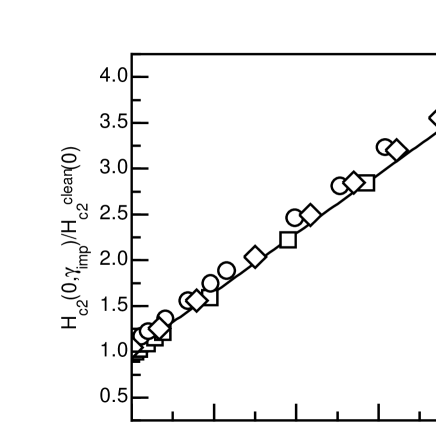
FIG. 2.: The calculated upper critical field for $\mu*$=0.13 and $\lambda=$1 ($\Box$), 2 ($\circ$), 3 ($\Diamond$) (Eqs. 1-5) normalized on its approximate clean limit value (Eq. 14) $vs$ normalized impurity scattering rate $\gamma_{imp}/T_{c}(1+\lambda)$. Solid line indicates BCS approximation (Eq. 20).

One realizes that this simple BCS-type relationship holds in the moderate strongly coupled case, too.

To summarize, for nearly isotropic single band metals the upper critical field at low temperature can be estimated with high accuracy by rather simple semi-analytical formulas Eqs. (12-15) and Eq. (20).

A An instructive example from MgB₂

Recently Manske et al. [16] suggested that experimental data for the novel superconductor MgB₂ which we interpreted in terms of a multi-component gap approach [9], can be also described within the standard isotropic single-band Eliashberg model using Eq. (12). They reported 2$\Delta_{0}/k_{B}T_{c}\approx 4.1$ and H${}_{c2}(0)$= 14 T in seemingly good agreement with experimental data for $H_{c2}(0)$. The other reported quantities are $\omega_{ln}$=30 meV, $T_{c}$=30 K. Using their input (material) parameters presented in that paper we checked their calculations and find that their model gives actually $\omega_{ln}$=53 meV, $T_{c}$=26 K, 2$\Delta_{0}/k_{B}T_{c}=$3.8, and $H_{c2}(T=0)$ = 1.2 T in sharp contrast with their set mentioned above. Thus, at first, we confirm our earlier result [9] that the standard ISB model can not be applied to MgB₂. At second, we note that the use of formulas written in practical units might be helpful to avoid such incorrect estimations.