Large-$S$ approach to chiral phases in frustrated spin chains

1 Introduction

Chirally ordered phases in frustrated quantum spin chains have attracted considerable attention recently [1, 2, 3, 4, 5, 6, 7, 8, 9]. Nersesyan et al.[1] have studied the antiferromagnetic $S={1\over 2}$ chain with easy-plane anisotropy and frustrating next-nearest-neighbor (NNN) coupling, described by the Hamiltonian

$$\widehat{H}=\sum_{n}\{({\mathbf{S}}_{n}{\mathbf{S}}_{n+1})_{\mathchar 28929\relax}+j({\mathbf{S}}_{n}{\mathbf{S}}_{n+2})_{\mathchar 28929\relax},\quad({\mathbf{S}}_{1}{\mathbf{S}}_{2})_{\mathchar 28929\relax}\equiv S_{1}^{x}S_{2}^{x}+S_{1}^{y}S_{2}^{y}+\mathchar 28929\relax S_{1}^{z}S_{2}^{z}\,,$$ (1.1)

where ${\mathbf{S}}_{n}$ denotes the spin operator at the $n$-th site, $j>0$ is the relative strength of the NNN coupling, and $0<\mathchar 28929\relax<1$ is the dipolar easy-plane anisotropy. In the limit $j\gg 1$, performing the Abelian bosonization and subsequently using RG and mean-field arguments, they have predicted the existence of a new gapless phase with a broken parity, which is characterized by the nonzero value of the vector chirality ${\mathbf{\kappa}}_{n}=\langle({\mathbf{S}}_{n}\times{\mathbf{S}}_{n+1})\rangle$. This type of ordering does not break the U(1) in-plane rotation symmetry, it only breaks the discrete parity symmetry and thus is in principle perfectly allowed in one dimension, the idea probably first realized by Chubukov. [10] Except having the chiral order, this phase is characterized by the power-law decaying incommensurate in-plane spin correlations of the form $\langle S^{+}_{0}S^{-}_{n}\rangle\propto n^{-\eta}e^{iQn}$, where $Q$ is very close to $\pi$ in the limit $j\gg 1$, and $\eta={1\over 4}$ for $S={1\over 2}$.[1]

Early attempts [2, 4] to find this chiral gapless phase in numerical calculations for $S={1\over 2}$ were unsuccessful. At the same time, to much of surprise, DMRG studies for frustrated $S=1$ chain [2, 5] have shown the presence of two different types of chiral phases, gapped and gapless. Later, chiral phases were numerically found for $S={1\over 2}$, [7, 8] as well as for $S={3\over 2}$ and $S=2$. [8]

For general $S$, the appearance of two chiral phases was explained with the help of the large-$S$ mapping to a helimagnet, and the qualitative form of the phase diagram for large $S$ was given.[6] However, the way of mapping to a helimagnet used in Ref. [6] neglects the presence of the topological term and thus is in fact valid only for integer $S$, when the topological term is ineffective.

Another theoretical approach using bosonization [9] suggests that the phase diagram for integer and half-integer $S$ should be very similar, with the only difference that the Haldane phase gets replaced by the dimerized phase in the case of half-integer $S$. This is, however, in contradiction with the recent numerical results [8] indicating that the chiral gapped phase is absent for half-integer $S$.

In the present paper I show that the difference between integer and half-integer $S$, well known for small $j$, [12] persists also for the chiral region of the phase diagram, which leads to disappearance of the chiral gapped phase and also changes dramatically the mechanisms of destabilization of the chiral gapless phase.

2 Modified nonlinear sigma model

Consider the model (1.1) for general (large) spin $S$. One can pass to the spin coherent states in a usual manner, as described, e.g., in Ref. [11]. The Berry phase for a single spin at the site $i$ can be expressed through the unit vector $\vec{n}_{i}$ parametrizing the coherent state: $\mathchar 28936\relax_{i}=S\int dt\,{\partial_{t}\vec{n}_{i}\cdot(\vec{n}_{i}\times\vec{e}_{i})\over 1+\vec{n}_{i}\cdot\vec{e}_{i}}$, where $\vec{e}$ is an arbitrary unit vector. If we choose $\vec{e}_{1}=-\vec{n}_{2}$ and $\vec{e}_{2}=-\vec{n}_{1}$, the sum of Berry phases for two neighboring spins at sites $1$ and $2$ can be written easily in a compact form : $\mathchar 28936\relax_{12}=S{\vec{n}_{1}\times\vec{n}_{2}\over 1-\vec{n}_{1}\cdot\vec{n}_{2}}\cdot\partial_{t}(\vec{n}_{2}-\vec{n}_{1})$. Further, we select the uniform and staggered components of the magnetization, putting $\vec{n}_{i}=\vec{m}_{i}+(-1)^{i}\vec{l}_{i}$. When we are in the vicinity of the classical Lifshitz point $j={1\over 4}$, both uniform and staggered magnetization vary slowly in space, so that we can pass to the continuum approximation, assuming as usual that $m\ll l$. The effective action is readily obtained in the following form:

$${\cal A} = 2\pi SQ+S\int dx\int dt\,\vec{m}(\vec{l}\times\partial_{t}\vec{l})$$

$$- S^{2}\int dx\int dt\,{\hbox{$\left\{\vbox to0.0pt{}\right.\n@space$}}{3\over 4}(1-\mathchar 28929\relax)l_{z}^{2}+2f_{\alpha}m_{\alpha}^{2}-2\varepsilon h_{\alpha}(\partial_{x}l_{\alpha})^{2}+{1\over 8}h_{\alpha}(\partial^{2}_{xx}l_{\alpha})^{2}{\hbox{$\left\}\vbox to0.0pt{}\right.\n@space$}}\,,$$

where $Q={1\over 4\pi}\int dt\int dx\vec{l}\cdot(\partial_{x}\vec{l}\times\partial_{t}\vec{l})$ is the topological charge, and we use the notation

$$\varepsilon=j-1/4,\quad f_{x,y}=h_{x,y}=1,\quad f_{z}=(3+5\mathchar 28929\relax)/8,\quad h_{z}=\mathchar 28929\relax.$$ (2.2)

For the sake of clarity, we have set the Planck constant and the lattice constant to unity. Making Taylor expansions of the fields, one has to take into account the derivatives of $\vec{l}$ up to the fourth order, since, as one can see from (2), the contribution of the second order comes with the prefactor $\varepsilon$ which becomes negative in the region $j>{1\over 4}$ we are interested in. Note also that we do not assume $\mathchar 28929\relax$ to be close to $1$ and thus have to keep terms like $(1-\mathchar 28929\relax)$ multiplied by $m_{z}^{2}$ or $(\partial_{x}l_{z})^{2}$ etc. The uniform part $\vec{m}$ can be integrated out, and after passing to the imaginary “time” $\tau=2iSt$ one obtains the following effective Euclidean action, valid in the vicinity of the Lifshitz point:

$${\cal A}_{E} = {1\over 2g_{0}}\int dx\int d\tau{\hbox{$\left\{\vbox to0.0pt{}\right.\n@space$}}{1\over f_{\alpha}}(\vec{l}\times\partial_{\tau}\vec{l})_{\alpha}^{2}-4\varepsilon\,h_{\alpha}(\partial_{x}l_{\alpha})^{2}+{1\over 4}\,h_{\alpha}\,(\partial^{2}_{xx}l_{\alpha})^{2}$$ (2.3)

$$+ {3\over 2}(1-\mathchar 28929\relax)(l_{z})^{2}{\hbox{$\left\}\vbox to0.0pt{}\right.\n@space$}}+i2\pi SQ,$$

where the bare coupling constant $g_{0}=2/S$. It is easy to see that for $\mathchar 28929\relax\to 1$ and $j\to 0$ the action (2.3) gives the well-known expression for the isotropic Heisenberg chain (the fourth-order derivatives become irrelevant in this limit).

3 Mapping to a helimagnet

Now I will show that the action (2.3) can be further mapped to a helimagnet, giving the results very similar to those obtained with the help of the ansatz of Ref. [6]. Passing to the angular variables $l_{x}+il_{y}=\sin\theta e^{i\varphi}$, $l_{z}=\cos\theta$, one may notice that for $\mathchar 28929\relax\not=1$ the field $\theta$ is massive, and thus can be integrated out. Putting $\theta={\pi\over 2}+\vartheta$ and expanding in $\vartheta$, one can rewrite the action as

$${\cal A}_{E} = {\cal A}[\vartheta]+{1\over 2g_{0}}\int dx\int d\tau{\hbox{$\left\{\vbox to0.0pt{}\right.\n@space$}}{1\over f_{z}}(\partial_{\tau}\varphi)^{2}[1+(f_{z}-2)\vartheta^{2}]$$ (3.1)

$$+ (1-\vartheta^{2}){\hbox{$\left[\vbox to0.0pt{}\right.\n@space$}}-4\varepsilon(\partial_{x}\varphi)^{2}+{1\over 4}(\partial_{x}\varphi)^{4}+{1\over 4}(\partial^{2}_{xx}\varphi)^{2}{\hbox{$\left]\vbox to0.0pt{}\right.\n@space$}}{\hbox{$\left\}\vbox to0.0pt{}\right.\n@space$}}+i2\pi SQ,$$

$${\cal A}[\vartheta] = {1\over 2g_{0}}\int dx\int d\tau{\hbox{$\left\{\vbox to0.0pt{}\right.\n@space$}}(\partial_{\tau}\vartheta)^{2}-4\varepsilon\mathchar 28929\relax(\partial_{x}\vartheta)^{2}+{1\over 4}\mathchar 28929\relax(\partial^{2}_{xx}\vartheta)^{2}-{3\over 2}(1-\mathchar 28929\relax)\vartheta^{2}{\hbox{$\left\}\vbox to0.0pt{}\right.\n@space$}}$$

Further, introducing instead of $\vartheta$ a new variable $\xi$ by putting $\vartheta={1\over 2}(\xi e^{i\lambda x}+\xi^{*}e^{-i\lambda x})$, where $\xi$ is assumed to be small and smoothly varying, one can obtain the action ${\cal A}[\xi]$ where now only quadratic terms in $\xi$ have to be kept. In order to kill terms of the type $\xi\partial_{x}\xi^{*}-\xi^{*}\partial_{x}\xi$, it is necessary to set $\lambda=\lambda_{0}$, where $\lambda_{0}=\sqrt{8\varepsilon}$ is the classical pitch of the helix in the limit $\varepsilon\ll 1$. The action now takes the form

$${\cal A}_{E} = \int dx\int d\tau{\hbox{$\left\{\vbox to0.0pt{}\right.\n@space$}}{1\over 2\widetilde{g_{0}}}(\partial_{\tau}\varphi)^{2}{\hbox{$\left[\vbox to0.0pt{}\right.\n@space$}}1+{1\over 2}(1+Z)|\xi|^{2}{\hbox{$\left]\vbox to0.0pt{}\right.\n@space$}}+{1\over 2g_{0}}{\hbox{$\left[\vbox to0.0pt{}\right.\n@space$}}1-{1\over 2}|\xi|^{2}{\hbox{$\left]\vbox to0.0pt{}\right.\n@space$}}V[\varphi]{\hbox{$\left\}\vbox to0.0pt{}\right.\n@space$}}$$ (3.2)

$$+ {\widetilde{E}\over g_{0}}\int dx\int d\widetilde{\tau}{\hbox{$\left\{\vbox to0.0pt{}\right.\n@space$}}|\partial_{\widetilde{\tau}}\xi|^{2}+|\partial_{x}\xi|^{2}+m_{0}^{2}|\xi|^{2}{\hbox{$\left\}\vbox to0.0pt{}\right.\n@space$}}+i2\pi SQ,$$

where the following notation is used:

$$\widetilde{g_{0}}=g_{0}(1-Z),\quad Z={5\over 8}(1-\mathchar 28929\relax),\quad m_{0}^{2}={3(1-\mathchar 28929\relax)\over 16\varepsilon\mathchar 28929\relax},\quad\widetilde{E}=\sqrt{{\varepsilon\mathchar 28929\relax\over 2}}$$

$$\widetilde{\tau}=\tau\sqrt{8\varepsilon\mathchar 28929\relax},\quad V[\varphi]={1\over 4}{\hbox{$\left[\vbox to0.0pt{}\right.\n@space$}}(\partial_{x}\varphi)^{2}-8\varepsilon{\hbox{$\left]\vbox to0.0pt{}\right.\n@space$}}^{2}+{1\over 4}(\partial^{2}_{xx}\varphi)^{2}.$$ (3.3)

Applying the standard Polyakov-type RG, one obtains finally the effective action of the planar helimagnet, which depends only on in-plane angle $\varphi$:

$${\cal A}[\varphi]={1\over 2T_{\rm eff}}\int dx\int dy{\hbox{$\left\{\vbox to0.0pt{}\right.\n@space$}}(\partial_{y}\varphi)^{2}+V[\varphi]{\hbox{$\left\}\vbox to0.0pt{}\right.\n@space$}}+i2\pi SQ,\quad T_{\rm eff}\equiv\sqrt{g\widetilde{g}},\quad y=\tau\sqrt{\widetilde{g}/g}$$

$$g={g_{0}\over 1-\displaystyle{g_{0}\over 8\pi\widetilde{E}}\ln(1+\mathchar 28931\relax_{0}^{2}/m_{0}^{2})},\quad\widetilde{g}={\widetilde{g_{0}}\over 1-\displaystyle{\widetilde{g_{0}}\over 8\pi\widetilde{E}}{1+Z\over 1-Z}\ln(1+\mathchar 28931\relax_{0}^{2}/m_{0}^{2})},$$ (3.4)

here $\mathchar 28931\relax_{0}=\pi$ is the momentum cutoff on the lattice. The problem is thus mapped to the classical helimagnet in two dimensions at the finite temperature $T_{\rm eff}$.

One may notice that we have kept the topological term in (3), although formally we don’t have the right to do that after mapping to the planar model. Keeping this term is, however, important for the following discussion, if one considers singular configurations like vortices: In the vortex core the planar mapping becomes invalid, since the angle $\theta$ deviates there strongly from $\pi/2$.

4 Phase transitions

The action (3) is very similar to that derived in Ref. [6] (although slightly different in detail), and we will see that it yields exactly the same results concerning the transition lines.

The transition from gapless chiral to gapped chiral phase is determined by the unbinding of vortices existing on the background of a state with a certain chirality. The critical “temperature” of this transition can be obtained by rewriting the action (3) in terms of deviation from the ground state with a certain chirality, i.e., setting $\varphi=\lambda_{0}x+\phi$. Then one may neglect the higher-order terms in derivatives of $\phi$ and get the classical $XY$ action of the form

$${\cal A}={1\over 2T_{\rm eff}}\int\!\!\int\!\!dx\,dy\,{\hbox{$\left\{\vbox to0.0pt{}\right.\n@space$}}(\partial_{y}\phi)^{2}+\lambda_{0}^{2}(\partial_{x}\phi)^{2}{\hbox{$\left\}\vbox to0.0pt{}\right.\n@space$}},$$

from which the critical $T_{\rm eff}$ is given by the equation

$$T_{\rm eff}^{KT}=(\pi/2)\lambda_{0}$$ (4.1)

For $\varepsilon\to 0$ and finite (not very small) anisotropy $1-\mathchar 28929\relax$ one has $g\simeq g_{0}$, $\widetilde{g}\simeq\widetilde{g_{0}}$, and (4.1) translates into

$$\varepsilon_{KT}=(3+5\mathchar 28929\relax)/4\pi^{2}S^{2}$$ (4.2)

exactly the result given in Ref. [6]. In the other limit, when $1-\mathchar 28929\relax\to 0$ and $\varepsilon$ is small but finite, one may neglect the difference between $g$ and $\widetilde{g}$, which yields the following equation for the transition line:

$$(1-\mathchar 28929\relax)_{KT}=(16/3)\varepsilon\mathchar 28931\relax_{0}^{2}\exp\{-2(\pi S\sqrt{2\varepsilon}-2)\},$$ (4.3)

again the result coinciding with that previously obtained.[6]

The in-plane correlation function in the KT (gapless chiral) phase can be readily obtained and has the power-law form

$$\langle S^{+}(x)S^{-}(0)\rangle\propto x^{-\eta}\,e^{i(\pi\pm\lambda_{0})x},\quad\eta=T_{\rm eff}/(2\pi\lambda_{0})\to{1\over 8\pi S}\sqrt{{3+5\mathchar 28929\relax\over\varepsilon}},\;\;\varepsilon\to 0\,.$$ (4.4)

The critical exponent $\eta$ increases when one approaches the transition; this behavior of $\eta$ is in qualitative agreement with the numerical results[8], see Fig. 4. One should mention, however, that the estimated numerical values of $\eta$ are not universal at the transition boundary, while the picture advocated here would imply the universal KT value of $\eta={1\over 4}$. Further studies are necessary to clarify this point. The large-$j$ behavior of $\eta$, which is not accessible by the present approach, was studied by Lecheminant et al. within the bosonization framework,[9] and the predicted value $\eta(j\to\infty)=1/8S$ is in a good agreement with the numerical data.[8]

The temperature of the transition between chiral and non-chiral phases can be estimated in a “solid-on-solid” approximation [13] by considering the fluctuations of a chiral domain wall.[6] Any such fluctuation requires formation of topological defects with nonzero vorticity, as shown in Fig. 2.

Fig. 2: A schematic view of the elementary “fluctuation” in a chiral domain wall: an instanton connecting two domain wall states separated by the minimum possible distance $\pi/\lambda_{0}$ (displacement by one “quantum”). The instanton necessarily includes a vortex-like topological defect and thus has the topological charge $Q=\pm{1\over 2}$. The dashed line indicates the position of the domain wall.

Such field configurations, which we will call “bound vortices”, are instantons connecting states with different positions of the domain wall in space, and the corresponding change in the position is quantized in multiples of $\pi/\lambda_{0}$. The free energy $\sigma$ of the domain wall per unit length in the $y$ direction can be written as

$$\sigma=E_{DW}-{T_{\rm eff}\over L}\ln{\cal Z},\quad{\cal Z}=\sum_{N=0}^{N_{0}}\int_{y_{N-1}}^{L}dy_{N}\cdots\int_{0}^{y_{2}}dy_{1}\sum_{\{n_{i}\not=0\}}e^{\displaystyle-{E_{bv}\over T_{\rm eff}}\sum_{i=1}^{N}|n_{i}|},$$ (4.5)

where $L$ is the length of the domain wall, $E_{bv}$ is the energy of the bound vortex, $E_{DW}$ is the energy of the domain wall (per unit length), $N_{0}=L/d_{0}$, where $d_{0}$ is the minimal possible distance in $y$ direction between successive fluctuations, and the positions $y_{i}$ of fluctuations are subject to the constraint $|y_{i}-y_{i+1}|\leq d_{0}$. The multiple integral in (4.5) is easily calculated to be equal to $(L-Nd_{0})^{N}/N!$ by making the substitution $\zeta_{i}=y_{i}-(i-1)d_{0}$, and after applying the Stirling formula one finally gets

$$\sigma=E_{DW}-(T/d_{0})\ln{\hbox{$\left\{\vbox to0.0pt{}\right.\n@space$}}1+d_{0}{\hbox{$\left(\vbox to0.0pt{}\right.\n@space$}}\mbox{cotanh}(E_{bv}/2T_{\rm eff})-1{\hbox{$\left)\vbox to0.0pt{}\right.\n@space$}}{\hbox{$\left\}\vbox to0.0pt{}\right.\n@space$}}$$ (4.6)

Fig. 1: Behavior of the critical exponent $\eta$ of the in-plane correlations in the chiral gapless phase (see Eq. (4.4)) as a function of $j$. Solid and dashed lines are the results of present approach for $S=1$ and $S=2$, respectively, and circles and squares are numerical results for $S=1$ and $S=2$ taken from Ref. [8].

 

We cannot calculate the energy of the bound vortex $E_{bv}$ and the scale $d_{0}$ analytically. Assuming that bound and free vortex solutions have similar structure apart from the core region, and cutting the free vortex solution at the distance $\pi/\lambda_{0}$, one may estimate $E_{bv}\simeq\pi\lambda_{0}\ln(\pi/\lambda_{0})$ and $d_{0}=\pi/\lambda_{0}^{2}$. Then the equation $\sigma=0$ can be solved numerically, and the corresponding solution $T_{\rm eff}^{I}$ as a function of $j$ for $j\to 1/4$ is shown in Fig. 4 together with the corresponding critical temperature of the Kosterlitz-Thouless transition. One can see that the two temperatures are very close to each other, but $T^{I}$ is slightly higher than $T^{KT}$.

Thus, for integer $S$ we obtain the same phase diagram as suggested in Ref. [6]. Now, the question is what changes in this picture if $S$ becomes half-integer?

As it was mentioned before, the planar description becomes invalid near the vortex core, where it becomes energetically favorable to lift the spins from the easy plane in order to reduce the contribution of the gradient terms in the action. The vector $\vec{l}$ in the center of a vortex is in fact perpendicular to the plane, and thus the vortices present in the model are in fact not $Z$ vortices of the purely $XY$ system, but rather $Z_{2}$ vortices of the Heisenberg model. The topological charge of a vortex is $Q=-p\nu/2=\pm{1\over 2}$, where $p=\pm 1$ is the sign of $\cos\theta$ in the vortex center, and $\nu=\pm 1$ is the usual $XY$ vorticity (the angle $\varphi$ changes by $2\pi\nu$ when one goes around the center). Therefore, for half-integer $S$ every vortex obtains the effective phase factor $e^{i2\pi SQ}=e^{\pm i\pi/2}$, and after summation over possible values of $Q$ the contribution of vortices vanishes. This has the usual consequence of suppressing the Kosterlitz-Thouless transition, which disappears for half-integer $S$ also for small $j$, together with the corresponding gapped (Haldane) phase. [12] Thus one may expect that only the chiral gapless phase should survive for half-integer $S$, in accordance with the numerical results. [8]

Fig. 3: The effective critical “temperatures” $T_{\rm eff}$ of the Ising (chiral — non-chiral) and Kosterlitz-Thouless (chiral gapless — chiral gapped) transitions, according to Eqs. (4.1) and (4.6). One can see that the region of existence of the chiral gapped phase is very narrow.

 

Another, somewhat unexpected, effect of the topological term is that it suppresses the fluctuations of the chiral domain walls as well. Indeed, since every elementary fluctuation (a “jump” by $\pi/\lambda_{0}$ in space) contains a “bound vortex”, the contribution of configurations with $n_{i}\not=0$ in (4.5) should vanish. That means that the mechanisms of destabilizing the chiral gapless phase for integer and half-integer $S$ must be very different. At present, I am not able to suggest any efficient mechanism for destroying the chiral phase for half-integer $S$. One may speculate that high-energy configurations with discontinuities may play some role (an example of such configuration is shown in Fig. Large-$S$ approach to chiral phases in frustrated spin chains). Another possibility would be that due to interaction between bound vortices the energy of configurations describing the domain wall fluctuations with even $n_{i}$ will be the lowest when all $n_{i}$ “bound vortices” have the same topological charge $Q=+{1\over 2}$ or $-{1\over 2}$ (note that a uniform sequence of $Q$ means an alternating sequence of $p=\mbox{sign}{\cos\theta}$, since the vorticities $\nu$ must alternate). In any case, such explanations would mean a strong increase of the Ising transition temperature in comparison to the integer $S$ case.

Acknowledgments. — I would like to thank P. Azaria, T. Hikihara, T. Jolicoeur, C. Lhuillier, and P. Lecheminant for the fruitful discussions on the subject. This work was partly supported by Volkswagen-Stiftung through Grant I/75895.

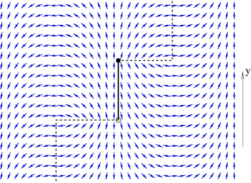
Fig. 4: An example of configuration with discontinuity which may contribute to the destabilization of the chiral gapless phase for half-integer $S$, see the text. The dashed line shows the position of the chiral domain wall, and the discontinuity is indicated by the solid line. The discontinuity is a chiral domain wall with an additional $\pi$ phase jump; at both ends of the discontinuity there are “half-vortices” which carry the topological charge $Q=\pm{1\over 4}$.

References

• [1] A. A. Nersesyan, A. O. Gogolin, and F. H. L. Eßler, Phys. Rev. Lett. 81 (1998), 910.
• [2] M. Kaburagi, H. Kawamura, and T. Hikihara, J. Phys. Soc. Jpn. 68 (1999), 3185.
• [3] D. Allen and D. SΓ©nΓ©chal, Phys. Rev. B 61 (2000), 12134.
• [4] A. A. Aligia, C. D. Batista, and F. H. L. Eßler, Phys. Rev. B 62 (2000), 6259.
• [5] T. Hikihara, M. Kaburagi, H. Kawamura, and T. Tonegawa, J. Phys. Soc. Jpn. 69 (2000), 259.
• [6] A. K. Kolezhuk, Phys. Rev. B 62 (2000), R6057.
• [7] Y. Nishiyama, Eur. Phys. J. B 17 (2000), 295.
• [8] T. Hikihara, M. Kaburagi, and H. Kawamura, Phys. Rev. B 63 (2001), 174430.
• [9] P. Lecheminant, T. Jolicoeur, P. Azaria, Phys. Rev. B 63 (2001), 174426.
• [10] A. V. Chubukov, Phys. Rev. B 44 (1991), 4693.
• [11] E. Fradkin, Field Theories of Condensed Matter Systems (Addison-Wesley, Reading, 1991).
R. Manousakis, Rev. Mod. Phys. 63 (1991), 1.
• [12] See, e.g., I. Affleck, J. Phys.: Cond. Matter 1 (1989), 3047 and references therein.
• [13] E. MΓΌller-Hartmann and J. Zittartz, Z. Phys. B 27 (1977), 261.
Refer to caption