Stable Magnetostatic Solitons in Yttrium Iron Garnet Film Waveguides for Tilted in-Plane Magnetic Fields

Abstract

The possibility of nonlinear pulses generation in Yttrium Iron Garnet thin films for arbitrary direction between waveguide and applied static in-plane magnetic field is considered. Up to now only the cases of in-plane magnetic fields either perpendicular or parallel to waveguide direction have been studied both experimentally and theoretically. In the present paper it is shown that also for other angles (besides 0 or 90 degrees) between a waveguide and static in-plane magnetic field the stable bright or dark (depending on magnitude of magnetic field) solitons could be created.

I Introduction

The investigation of magnetostatic envelope solitons in yttrium-iron garnet thin magnetic films is one of the ”hot topics” in nowadays physics. The advanced instrumentation for microwave pulse generation, detection and analysis together with the solid theoretical base has led to a growing interest in studying such localized objects. The definition ”magnetostatic soliton” refers to a propagating pulse formed by large wavelength spin excitations which do not ”feel” the exchange interaction and only the dipolar interactions could be taken into account. Thus the processes are characterized by the Landau-Lifshitz and magnetostatic equations.

The linearized solutions of these equations were obtained by Damon and Eshbach damon 40 years ago for arbitrary direction between wave vector of spin excitations and in-plane magnetic field. The nature of those excitations has been also studied experimentally hurben . The weakly nonlinear limit for the mentioned equations also was considered for the particular cases when wave vector of spin excitations is either parallel (backward volume waves) or perpendicular (surface waves) to the direction of in-plane magnetic field. It was found out zvezdin that the envelope of spin excitations in both cases satisfy 2D Nonlinear Schrödinger (NLS) equation which permits well-known 1D soliton solutions depending on the relative sign of dispersion and nonlinear terms.

In full accordance with the theoretical predictions the bright solitons have been observed for nonlinear backward volume waves case boyle - xia (in-plane field is directed parallel to the carrier wave vector and propagation velocity of envelope soliton), while the dark solitons are created in case of nolinear surface waves chen2 -kalinikos (carrier wave vector and group velocity is perpendicular to the magnetic field). It should be especially noted that all the mentioned solitons are observed in narrow strips. In such geometries the transverse instabilities do not develop and experiments show the stable propagation of 1D solitons along the waveguides. At the same time, in wide samples 1D solitons are in general unstable zakharov , kivshar and form metastable spin wave bullets which decay either after edge reflection or mutual interaction zalit1 , zalit2 .

We emphasize that the solitons in in-plane magnetized films are studied both theoretically and experimentally only for two particular cases when the pulse propagates along or perpendicular to the magnetic field. Only very recently the general case of linear and nonlinear magnetostatic wave propagation in wide samples was investigated ref for a wide range of angles between propagation velocity and magnetic field. In this connection the natural question arises: why one does not consider the nonlinear pulses in waveguides which are not either parallel or perpendicular to in-plane static magnetic field. As we show below for each magnitude of internal magnetic field it is possible to choose the direction (besides 0 or 90 degrees) of waveguide respect to magnetic field direction for which stable propagation of envelope solitons is allowed (see inset of Fig. 1 for a geometry of the problem). We determine the limits for magnitude of magnetic field, angle between waveguide and magnetic field vector and pulse frequency necessary for creation of dark or bright envelope solitons. We also calculate their widths and propagation velocities and claim that such solitons could be experimentally observed.

II Basic Consideration: Linear Magnetostatic Waves

The linear consideration is based upon the Damon-Eshbach formulation damon and its generalization by Hurben and Patton hurben for the case of arbitrary angles between a wave vector $\vec{k}$ and static internal magnetic field $\vec{H}_{0}$. Further we will examine only so-called ”near-uniform” case ($kd\ll 1$, $d$ stands for a film thickness) and derive the dispersion expansion over the parameter $kd$ up to a second order. Therefore we present here only the steps necessary for this purpose. Consideration of the mentioned wave number range sufficiently simplifies calculations and, besides that, most of the experiments on the magnetostatic envelope solitons are made having such carrier wave numbers.

Examining an in-plane magnetized ferromagnetic film with unpinned surface spins let us make the following definitions: $z$ is a direction of internal static magnetic field; $\vec{r}$ indicates the radius vector lying in the sample plane ($y,~{}z$) and $x$ is a coordinate along the direction perpendicular to the film plane. Then one can write down the Landau-Lifshitz and magnetostatic equations:

$$\frac{d{\vec{M}}}{dt}=-g[{\vec{M}}\times{\vec{H}}]\qquad div({\vec{H}}+4\pi{\vec{M}})=0\qquad rot{\vec{H}}=0.$$ (1)

Here $g$ is a modulus of the gyromagnetic ratio for electrons; $\vec{M}$ is a magnetization density vector and $\vec{H}$ is an internal total magnetic field. Introducing dynamical dimensionless quantities $\vec{m}=(\vec{M}-\vec{M}_{0})/M_{0}$ and $\vec{h}=(\vec{H}-\vec{H}_{0})/H_{0}$ the following equations are obtained in the linear limit over $|\vec{m}|$:

$$\frac{dm_{x}}{dt}=\omega_{H}(m_{y}-h_{y});\qquad\frac{dm_{y}}{dt}=-\omega_{H}(m_{x}-h_{x});$$

$$\frac{\partial}{\partial x}\left(\omega_{H}h_{x}+\omega_{M}m_{x}\right)+\frac{\partial}{\partial y}\left(\omega_{H}h_{y}+\omega_{M}m_{y}\right)+\frac{\partial}{\partial z}\left(\omega_{H}h_{z}\right)=0,$$ (2)

where $\omega_{H}=gH_{0}$ and $\omega_{M}=4\pi gM_{0}$. Defining $\vec{h}=\vec{grad}\Phi$ and searching for the solution of Eq. (2) in periodical form over $t$ (i.e. $\Phi$ and $m_{x,y}$ being proportional to $exp(-i\omega t)$) we get:

$$\frac{\partial^{2}}{\partial z^{2}}\Phi+(\chi_{1}+1)\left(\frac{\partial^{2}}{\partial y^{2}}+\frac{\partial^{2}}{\partial x^{2}}\right)\Phi=0\qquad\mbox{for}\qquad|x|<\frac{d}{2},$$

$$\left(\frac{\partial^{2}}{\partial z^{2}}+\frac{\partial^{2}}{\partial y^{2}}+\frac{\partial^{2}}{\partial x^{2}}\right)\Phi=0\qquad\mbox{for}\qquad|x|>\frac{d}{2}$$ (3)

and

$$m_{x}=\frac{\omega_{H}}{\omega_{M}}\left(i\chi_{2}\frac{\partial\Phi}{\partial y}+\chi_{1}\frac{\partial\Phi}{\partial x}\right),\qquad m_{y}=-\frac{\omega_{H}}{\omega_{M}}\left(i\chi_{2}\frac{\partial\Phi}{\partial x}-\chi_{1}\frac{\partial\Phi}{\partial y}\right),$$

where

$$\chi_{1}=\frac{\omega_{H}\omega_{M}}{\omega_{H}^{2}-\omega^{2}},\qquad\chi_{2}=\frac{\omega\omega_{M}}{\omega_{H}^{2}-\omega^{2}}.$$

Thus from (3) we can write down a linear solution of (1) in the form hurben :

$$\Phi=\left(Ae^{\kappa x}+Be^{-\kappa x}\right)e^{-i(\omega t-\vec{k}\vec{r})}\qquad\mbox{for}\qquad|x|<\frac{d}{2};$$

$$\Phi=Ce^{-k(x-d/2)}e^{-i(\omega t-\vec{k}\vec{r})}\qquad\mbox{for}\qquad x>\frac{d}{2};$$ (4)

$$\Phi=De^{k(x+d/2)}e^{-i(\omega t-\vec{k}\vec{r})}\qquad\mbox{for}\qquad x<-\frac{d}{2},$$

where $A$, $B$, $C$ $D$ are arbitrary constants at the present stage,

$$\kappa^{2}=\frac{k^{2}+\chi_{1}k^{2}_{y}}{1+\chi_{1}}$$

and let us remind that two dimensional vectors $\vec{r}=(y,~{}z)$ and $\vec{k}=(k_{y},~{}k_{z})$ lye in the film plane and $k\equiv\sqrt{k_{y}^{2}+k_{z}^{2}}$.

If $\kappa^{2}>0$ we deal with a so-called surface mode, otherwise $\kappa=i\sqrt{-\kappa^{2}}$ and a volume mode exists. However, note that due to the condition of ”near-uniformity” $kd\ll 1$ the difference between these two modes is negligible.

The dispersion relation can be obtained from (4) if we remember about the boundary conditions. Particularly the functions $\Phi$ and $h_{x}+4\pi m_{x}$ should be continuous on the boundaries $-d/2$ and $d/2$ of the film. The dispersion relation for both modes could be written as follows:

$$2k(\chi_{1}+1)\kappa\frac{e^{\kappa d}+e^{-\kappa d}}{e^{\kappa d}-e^{-\kappa d}}-k_{y}^{2}\chi_{2}^{2}+k^{2}+\kappa^{2}(\chi_{1}+1)^{2}=0.$$ (5)

Working in the limit $kd\ll 1$ and keeping only the terms up to the second order of this parameter the following expression is obtained:

$$\omega=\omega_{0}+\frac{\omega_{M}}{4\omega_{0}}\frac{d}{k}\left(\omega_{M}k_{y}^{2}-\omega_{H}k_{z}^{2}\right)-\frac{\omega_{M}^{2}}{32\omega_{0}^{3}}\frac{d^{2}}{k^{2}}\left(\omega_{M}k_{y}^{2}-\omega_{H}k_{z}^{2}\right)^{2}+\frac{\omega_{M}}{4\omega_{0}}d^{2}\left(\omega_{H}\frac{k_{z}^{2}}{3}-\omega_{M}k_{y}^{2}\right),$$ (6)

where $\omega_{0}\equiv\omega(k=0)=\sqrt{\omega_{H}(\omega_{H}+\omega_{M})}$. Then we get from (6) the following expressions for the derivatives of $\omega$ over $k_{y}$ and $k_{z}$:

$$v_{y}=\frac{\partial\omega}{\partial k_{y}}=\frac{\omega_{M}}{4\omega_{0}}d\left\{\frac{k_{y}}{k}\left[\omega_{M}\frac{k_{y}^{2}}{k^{2}}+(2\omega_{M}+\omega_{H})\frac{k_{z}^{2}}{k^{2}}\right]+{\cal O}_{1}(kd)\right\},$$

$$v_{z}=\frac{\partial\omega}{\partial k_{z}}=-\frac{\omega_{M}}{4\omega_{0}}d\left\{\frac{k_{z}}{k}\left[\omega_{H}\frac{k_{z}^{2}}{k^{2}}+(2\omega_{H}+\omega_{M})\frac{k_{y}^{2}}{k^{2}}\right]+{\cal O}_{2}(kd)\right\},$$

$$\omega^{\prime\prime}_{yy}=\frac{\partial^{2}\omega}{\partial k_{y}^{2}}=\frac{\omega_{M}}{4\omega_{0}}\frac{d}{k}\left\{\frac{k_{z}^{2}}{k^{2}}\left[(2\omega_{M}+\omega_{H})\frac{k_{z}^{2}}{k^{2}}-(2\omega_{H}+\omega_{M})\frac{k_{y}^{2}}{k^{2}}\right]+{\cal O}^{\prime}_{1}(kd)\right\},$$

$$\omega^{\prime\prime}_{zz}=\frac{\partial^{2}\omega}{\partial k_{z}^{2}}=\frac{\omega_{M}}{4\omega_{0}}\frac{d}{k}\left\{\frac{k_{y}^{2}}{k^{2}}\left[(2\omega_{M}+\omega_{H})\frac{k_{z}^{2}}{k^{2}}-(2\omega_{H}+\omega_{M})\frac{k_{y}^{2}}{k^{2}}\right]+{\cal O}^{\prime}_{2}(kd)\right\},$$

$$\omega^{\prime\prime}_{yz}=\frac{\partial^{2}\omega}{\partial k_{z}k_{y}}=-\frac{\omega_{M}}{4\omega_{0}}\frac{d}{k}\left\{\frac{k_{y}k_{z}}{k^{2}}\left[(2\omega_{M}+\omega_{H})\frac{k_{z}^{2}}{k^{2}}-(2\omega_{H}+\omega_{M})\frac{k_{y}^{2}}{k^{2}}\right]+{\cal O}^{\prime}_{3}(kd)\right\}.$$ (7)

The higher approximation terms ${\cal O}_{j}(kd)$ and ${\cal O}^{\prime}_{j}(kd)$ are not presented here because of their rather cumbrous form, but we use them in the calculation as far as the leading terms in expressions (7) vanish in vicinity of some points, e.g. $k_{y}=0$ or $k_{z}=0$.

III Weakly Nonlinear Limit: Soliton Solutions

Defining a wave envelope $u$

$$m_{x}+im_{y}=u\cdot e^{-i(\omega t-\vec{k}\vec{r})}$$

and following the well known modulation approach karpman , zvezdin the nonlinear equation for wave envelope $u$ is derived (we redirect reader for details of obtaining this equation to the recent paper Ref. boyle where the full procedure is well described):

$$i\left(\frac{\partial u}{\partial t}+v_{y}\frac{\partial u}{\partial y}+v_{z}\frac{\partial u}{\partial z}\right)+\frac{\omega^{\prime\prime}_{yy}}{2}\frac{\partial^{2}u}{\partial y^{2}}+\frac{\omega^{\prime\prime}_{zz}}{2}\frac{\partial^{2}u}{\partial z^{2}}+\omega^{\prime\prime}_{yz}\frac{\partial^{2}u}{\partial y\partial z}-N|u|^{2}u=0.$$ (8)

All of the coefficients are defined by formulas (7) except the nonlinear coefficient $N$ which could be easily calculated taking into account that in nonlinear case we have a following identity:

$$\omega_{M}=4\pi gM_{0}m_{z}.$$

Then Substituting in (6) the expansion of $m_{z}$ in weakly nonlinear limit $m_{z}=1-|u|^{2}/2$ and using expression for $N$ from Refs. karpman , zvezdin , boyle we get in large wavelength limit ($kd\ll 1$)

$$N=\frac{\partial\omega}{\partial|u|^{2}}\biggr{|}_{k\rightarrow 0,~{}|u|\rightarrow 0}=\frac{\partial\omega_{0}}{\partial|u|^{2}}\biggr{|}_{|u|\rightarrow 0}=-\frac{\omega_{H}\omega_{M}}{4\omega_{0}}.$$ (9)

Let us mention that if carrier wave vector is parallel or perpendicular to the static internal magnetic field the coefficients $v_{y}$ and $w^{\prime\prime}_{yz}$ are equal to zero zvezdin , boyle . But for arbitrary angles between $\vec{k}$ and $\vec{H_{0}}$ that is not the case. Therefore we should introduce a new frame of references in order to vanish the nondiagonal term with coefficient $\omega^{\prime\prime}_{yz}$. This could be done rotating the frame of references $yz$ by the angle $\vartheta$

$$\xi=z\cos\vartheta+y\sin\vartheta,\qquad\eta=y\cos\vartheta-z\sin\vartheta,$$ (10)

where

$$tg2\vartheta=2\frac{\omega^{\prime\prime}_{yz}}{\omega^{\prime\prime}_{zz}-\omega^{\prime\prime}_{yy}}.$$ (11)

Then from (8) - (11) we obtain the following nonlinear equation:

$$i\left(\frac{\partial u}{\partial t}+v_{1}\frac{\partial u}{\partial\xi}+v_{2}\frac{\partial u}{\partial\eta}\right)+\frac{1}{2}R\frac{\partial^{2}u}{\partial\xi^{2}}+\frac{1}{2}S\frac{\partial^{2}u}{\partial\eta^{2}}-N|u|^{2}u=0,$$ (12)

where

$$R=\omega^{\prime\prime}_{zz}cos^{2}\vartheta+2\omega^{\prime\prime}_{zy}cos\vartheta\sin\vartheta+\omega^{\prime\prime}_{yy}sin^{2}\vartheta,$$

$$S=\omega^{\prime\prime}_{zz}sin^{2}\vartheta-2\omega^{\prime\prime}_{zy}cos\vartheta\sin\vartheta+\omega^{\prime\prime}_{yy}cos^{2}\vartheta,$$ (13)

$$v_{1}=v_{z}cos\vartheta+v_{y}sin\vartheta,\qquad v_{2}=v_{z}sin\vartheta-v_{y}cos\vartheta.$$ (14)

Afterwards in the moving frame of references

$$\xi_{1}=\xi-v_{1}t\qquad\eta_{1}=\eta-v_{2}t$$

we come to the 2D nonlinear Schrödinger equation:

$$i\frac{\partial u}{\partial t}+\frac{1}{2}R\frac{\partial^{2}u}{\partial\xi_{1}^{2}}+\frac{1}{2}S\frac{\partial^{2}u}{\partial\eta_{1}^{2}}-N|u|^{2}u=0$$ (15)

and can write down its 1D bright or dark soliton solutions assuming that soliton envelope is a function only of variables $\xi_{1}$ and $t$ (thus soliton propagates along a spatial axis $\xi$ with a velocity $v_{1}$). If $NR<0$ we have bright soliton with envelope

$$|u|=|u|_{max}sech\left\{\frac{\xi_{1}}{\Lambda}\right\},\qquad$$ (16)

while in case $NR>0$ dark soliton solution is permitted:

$$|u|=|u|_{max}\left|\frac{\sqrt{1-A^{2}}}{A}+i\cdot tanh\left\{\frac{\xi_{1}}{\Lambda}\right\}\right|,$$ (17)

where $A$ denotes the contrast of dark soliton (if $A=1$ one has a black dark soliton and gray dark otherwise) and soliton width $\Lambda$ is defined for both cases by the same way:

$$\Lambda=\left|\frac{R}{N}\right|^{1/2}\frac{1}{|u|_{max}},$$ (18)

Now we shall discuss the question about the stability of these 1D solitons.

IV Stable Solitons in Waveguides for Tilted Magnetic Fields

As well known 1D soliton solutions (16) and (17) of 2D NLS are not stable to the transverse modulations with wavenumbers $0<\kappa<\kappa_{c}$. According to the recent results (see e.g. Ref. kivshar ) $\kappa_{c}\sim 1/\Lambda$, thus, if the limits of transverse variable $\eta_{1}$ is less than soliton width the instabilities do not develop and 1D soliton solutions (16) and (17) would be stable. When one has fully spatial transverse variable $\eta_{1}$ the above condition means that narrow samples should be used. In our case we have the mixed variable $\eta_{1}=\eta-v_{2}t$ and therefore also the condition for time dependent part has to be introduced: $v_{2}t<\Lambda$ and in case

$$v_{2}=0$$ (19)

the transverse instabilities do not develop even for infinite time. Thus besides the condition (11) we get from (14) and (19) additional condition on the stable soliton parameters:

$$tg\vartheta=\frac{v_{y}}{v_{z}}.$$ (20)

Afterwards, in view of both conditions (14) and (20) we finally obtain the following equality:

$$\frac{\omega^{\prime\prime}_{yz}}{\omega^{\prime\prime}_{zz}-\omega^{\prime\prime}_{yy}}=\frac{v_{y}v_{z}}{v_{z}^{2}-v_{y}^{2}}.$$ (21)

Solving (21) as an expansion over small parameter $kd$ we simply come to the following expression for the angle $\varphi$ between carrier wavevector ${\vec{k}}$ and static magnetic field:

$$\sin\varphi=-\sqrt{\frac{\omega_{H}}{\omega_{H}+\omega_{M}}}\left(1+\frac{\omega_{M}(3\omega_{H}+\omega_{M})}{3(\omega_{H}^{2}-\omega_{M}^{2})}kd\right).$$ (22)

Obviously there exist also trivial solutions $\varphi=0$ and $\varphi=90^{o}$ which will not be considered as long as they correspond to the well studied cases of bright backward volume wave and dark surface wave solitons, respectively. Further using the condition (20) and definitions for dispersion coefficient (13) we get the expressions for $\vartheta$ and $R$ as functions of expansion parameter $kd$:

$$\sin\vartheta=\sqrt{\frac{\omega_{M}}{\omega_{M}+\omega_{H}}}\left(1-\frac{\omega_{H}}{\omega_{H}+\omega_{M}}kd\right);\qquad R=\frac{\omega_{M}(\omega_{M}-\omega_{H})}{2\sqrt{\omega_{H}(\omega_{M}+\omega_{H})}}\frac{d}{k}.$$ (23)

As long as the nonlinear coefficient $N$ according to (9) is always negative the possibility of appearance of dark or bright solitons depends on the sign of dispersion coefficient $R$. In view of the second relation in (23) we can conclude that bright solitons appears if $\omega_{H}<\omega_{M}$ while dark solitons could be created for larger magnetic fields $\omega_{H}>\omega_{M}$. From Exps. (18) and (6) we are also able to get the expressions for soliton width and detuning of pulse frequency, respectively:

$$\Lambda=\frac{d}{|u|_{max}}\sqrt{\frac{2|\omega_{M}-\omega_{H}|}{\omega_{H}kd}};\qquad\omega-\omega_{0}=\frac{\omega_{M}}{3}\sqrt{\frac{\omega_{M}}{\omega_{H}+\omega_{M}}}\frac{\omega_{M}}{\omega_{H}-\omega_{M}}(kd)^{2},$$ (24)

while the soliton propagation velocity could be given by simple approximate formula:

$$v\equiv v_{1}\simeq\frac{\omega_{M}d}{2}\sqrt{\frac{\omega_{M}}{\omega_{M}+\omega_{H}}}$$ (25)

It should be noted that our perturbative approach violates if $\omega_{H}\rightarrow\omega_{M}$. Besides that, we have a following restriction on the internal static magnetic field: $\omega_{H}>0.3\omega_{M}$. Otherwise the threshold for three magnon processes is reached and localized nonlinear wave will decay rapidly zvezdin .

As we see all of the quantities $\vartheta$, $\omega-\omega_{0}$ and $\Lambda$ specifying the soliton are the functions of $kd$ and $h=\omega_{H}/\omega_{M}$. Thus it is possible to plot $\omega-\omega_{0}$ and $\Lambda$ as the functions of $\vartheta$ for different $h$ (see Figs. 1 and 2).

In Fig. 1 we present how to choose the sample geometry (in other words how to choose an angle $\vartheta$ between waveguide and static magnetic field) and frequency of applied pulse for various $h\equiv\omega_{H}/\omega_{M}$ in order to create bright or dark soliton. While in Fig. 2 we show the dependence of soliton width on the geometry of the problem and static magnetic field. In both cases the curves are limited because of restriction of ”near uniformity” $kd\ll 1$ and the following parameters for YIG film are used: $d=10\mu m$ and $\omega_{M}=1750$ Oe. Note that bright solitons appear when the angle between waveguide and static magnetic field is less than 45^o. Besides that, the detuning of pulse should be positive in order to create dark solitons. For the purpose to create bright solitons the angles should be larger than $45^{o}$ and detuning has to be negative.

V Conclusions and Possible Experimental Setup

Summarizing we can declare that the possibility of stable magnetostatic soliton propagation in in-plane magnetized ferromagnetic films in presence of tilted (from waveguide direction) static in-plane magnetic fields is proved. The widths and velocities as well as the range of angles between waveguide and magnetic field is obtained for which the stable soliton propagation is allowed.

However, As it was mentioned by the anonymous referee the waveguide border (see dashed line in the inset of Fig. 1) could cause the reflection of carrier wave (wave vector $\vec{k}$) what will change the group velocity destructing thus the soliton. To avoid such a possibility we propose to use tube like magnetic waveguides (see Fig. 3). Then the carrier wave will not be reflected and, besides that, the condition of quasi-one dimensionality still holds. Let us make the following choice of the parameters of the problem: tube diameter $L=0.5$mm; film thickness $d=10\mu m$ and $1/L\ll k\ll 1/d$. Thus the near uniformity condition $kd\ll 1$ is still valid and simultaneously the consideration of the sample as locally flat is allowed proving thus approximate validity of solutions like Exp. (4).

Acknowledgements: We would like to thank Dr. David Tskhakaia for the guiding advice. R. Kh. acknowledges NSF-NATO award No DGE-0075191 providing the financial support for his stay in Oklahoma University where the paper was completed.

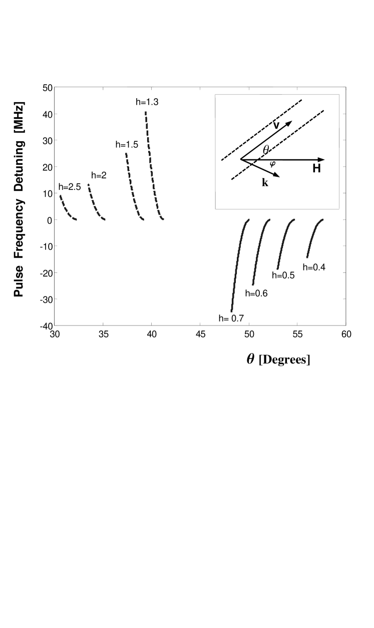
Figure 1: Detuning of the pulse frequency $\omega-\omega_{0}$ versus an angle $\theta$ between waveguide and static in-plane magnetic field for its different magnitude $h=\omega_{H}/\omega_{M}$. Dashed and solid lines correspond to the dark and bright soliton cases, respectively. Inset shows the geometry of the problem and dashed lines indicate the direction of a waveguide. The following film parameters are used in calculations: Film thickness $d=10\mu m$ and value of demagnetizing field $H_{M}=1750$ Oe.

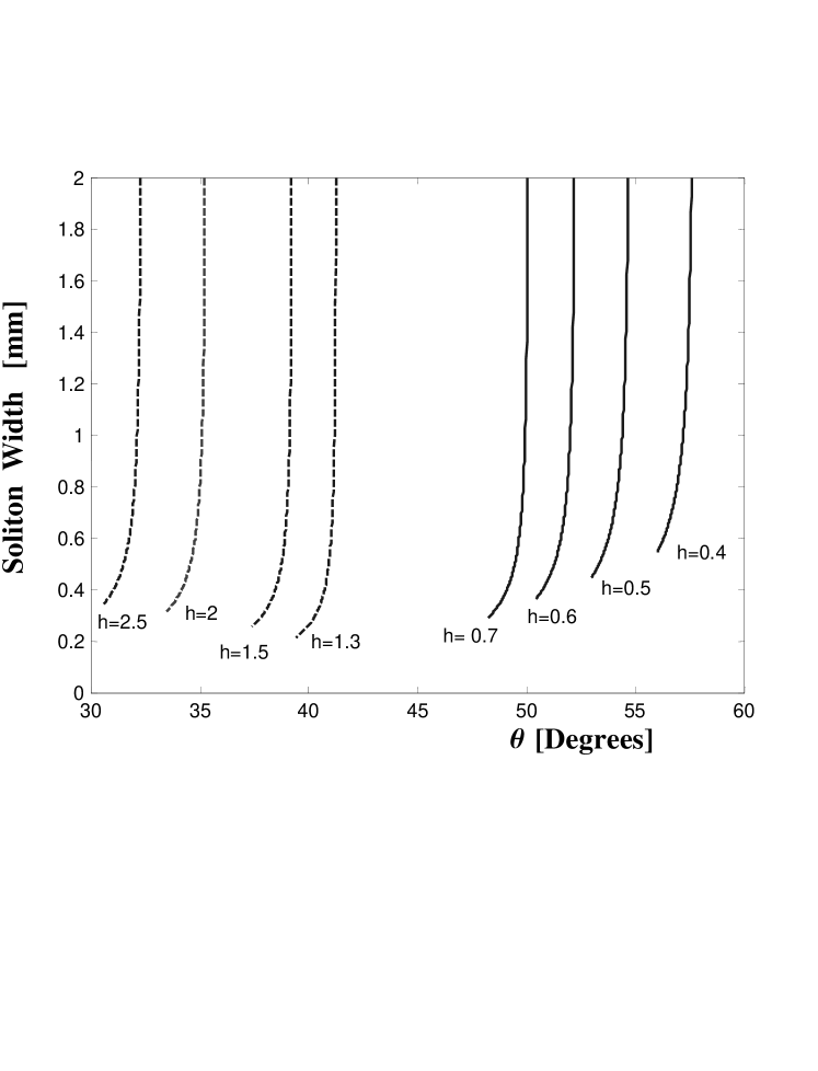
Figure 2: Dependence of the envelope soliton width on the angle $\theta$ between waveguide direction and in-plane magnetic field for its different value. Dashed and solid lines indicate dark and bright soliton cases, respectively. As in the previous figure $h=\omega_{H}/\omega_{M}$; $H_{M}=1750$ Oe; film thickness is equal to $d=10\mu m$ and, besides that, relative amplitude of soliton is taken as follows: $|u_{max}|=0.1$.

Figure 3: The possible experimental setup for observation of stable magnetostatic solitons. In each point of the sample magnetic field is parallel to the tube surface and tilted by the angle $\theta$ from the tube symmetry axis which is parallel to the envelope soliton propagation direction.

References

• (1) R.W. Damon, J.R. Eshbach, J. Phys. Chem. Solids, 19, 308, (1961).
• (2) M.J. Hurben, C.E. Patton, J. Magn. Magn. Mater., 139, 263, (1995).
• (3) A.K. Zvezdin, A.F. Popkov, Zh. Eksp. Theor Phys., 84, 606, (1983).
• (4) J.W. Boyle, S.A. Nikitov, A.D. Boardman, J.G. Booth, K. Booth, Phys.Rev.B., 53, 12173, (1996).
• (5) M. Chen, M.A. Tsankov, J.M. Nash, C.E. Patton, Phys.Rev.B., 49, 12773, (1994).
• (6) N.G. Kovshikov, B.A. Kalinikos, C.E. Patton, E.S. Wright, J.M. Nash, Phys.Rev.B., 54, 15210, (1996).
• (7) H. Xia, P. Kabos, C.E. Patton, H.E. Ensle, Phys.Rev.B., 55, 15018, (1997).
• (8) M. Chen, M.A. Tsankov, J.M. Nash, C.E. Patton, Phys. Rev. Lett., 70, 1707, (1993).
• (9) A.N. Slavin, Yu.S. Kivshar, E.A. Ostrovskaya, H. Benner, Phys. Rev. Lett., 82, 2583, (1999).
• (10) B.A. Kalinikos, M.M. Scott, C.E. Patton, Phys. Rev. Lett., 84, 4697, (2000).
• (11) V.E. Zakharov, A.M. Rubenchik, Zh. Eksp. Teor. Fiz., 65, 997, (1973); [Sov. Phys. JETP, 38, 494, (1974)].
• (12) Yu.S. Kivshar, D.E. Pelinovsky, Physics Reports, 331, 117, (2000).
• (13) M. Bauer, O. Büttner, S.O. Demokritov, B. Hillebrands, V. Grimalsky, Yu. Rapoport, A.N. Slavin, Phys. Rev. Lett., 81, 3769, (1998).
• (14) O. Büttner, M. Bauer, S.O. Demokritov, B. Hillebrands, M.P. Kostilev, B.A. Kalinikos, A.N. Slavin, Phys. Rev. Lett., 82, 4320, (1999).
• (15) O. Büttner, M. Bauer, S.O. Demokritov, B. Hillebrands, Yu.S. Kivshar, V. Grimalsky, Yu. Rapoport, A.N. Slavin, Phys. Rev. B, 61, 11576, (2000).
• (16) V.I. Karpman, Nonlinear Waves in Dispersive Media, Moskow, Nauka, (1970).
Refer to caption