Probability-Changing Cluster Algorithm for Two-Dimensional XY and Clock Models
Abstract
We extend the newly proposed probability-changing cluster (PCC) Monte Carlo algorithm to the study of systems with the vector order parameter. Wolff’s idea of the embedded cluster formalism is used for assigning clusters. The Kosterlitz-Thouless (KT) transitions for the two-dimensional (2D) XY and -state clock models are studied by using the PCC algorithm. Combined with the finite-size scaling analysis based on the KT form of the correlation length, , we determine the KT transition temperature and the decay exponent as and for the 2D XY model. We investigate two transitions of the KT type for the 2D -state clock models with , and for the first time confirm the prediction of at , the low-temperature critical point between the ordered and XY-like phases, systematically.
PACS numbers: 75.10.Hk, 64.60.Fr, 05.10.Ln
I Introduction
The two-dimensional (2D) XY model shows a unique phase transition, the Kosterlitz-Thouless (KT) transition [3, 4]. It does not have a true long-range order, but the correlation function decays as a power of the distance at all the temperatures below the KT transition point. José et al [5] studied the effect of the -fold symmetry-breaking fields on the 2D XY model; this is essentially the same as treating the -state clock model, where only the discrete values are allowed for the angle of the XY spins such that
| (1) |
In the limit we get the XY model. It was shown that the 2D -state clock model has two phase transitions of the KT type at and () for . There is an intermediate XY-like phase between a low-temperature ordered phase () and a high-temperature disordered phase (). It was predicted that the decay critical exponent varies from at to at .
Most of the above theoretical analyses relied on the renormalization group argument, and they are not exact. There have been extensive numerical studies on the 2D classical XY model [6, 7, 8, 9, 10, 11, 12]. In contrast, only a limited number of numerical works have been reported on the -state clock model [13, 14], and the accuracy was not good enough especially for the low-temperature phase transition. There have been no systematic studies to check the prediction of .
In numerical studies, efficient algorithms are important for getting the necessary information. The cluster update algorithms of the Monte Carlo simulation [15, 16] are examples of such efforts, and they are useful for overcoming the problems of slow dynamics. Recently we proposed an effective cluster algorithm, which is called the probability-changing cluster (PCC) algorithm, of tuning the critical point automatically [17]. It is an extension of the Swendsen-Wang algorithm [15], but we change the probability of cluster update (essentially, the temperature) depending on the observation whether clusters are percolating or not percolating. We showed the effectiveness of the PCC algorithm for the Potts models [17], determining the critical point and critical exponents for the second-order phase transition precisely with less numerical efforts. The PCC algorithm was also applied to the 2D site-diluted Ising model, where the crossover and the self-averaging properties were studied [18]. The advantage of using the PCC algorithm in the study of random systems is as follows: The sample-dependent for the finite system with the linear size is important for taking sample average, and the PCC algorithm is suitable for getting the sample-dependent .
There are a lot of interesting questions about the extension of the PCC algorithm. (i) Can the PCC algorithm be used for the problem of the vector order parameter, such as the XY model? (ii) Can it be applied to the analysis of the transition of the KT type? (iii) Can it work even if the system shows two or more phase transitions?
The purpose of the present paper is to answer these questions. We extend the PCC algorithm so as to treat systems with the vector order parameter. The rest of the paper is organized as follows. In Sec. II, we formulate the extension of the PCC algorithm for the vector order parameter. In Sec. III, the KT transition of the 2D XY model is studied with the finite-size scaling (FSS) analysis based on the KT form of the correlation length. In Sec. IV, we study the KT transitions of the 2D clock models. We investigate both phase transitions at and for the clock models. The summary and discussions are given in Sec. V.
II PCC algorithm for vector order parameter
Our Hamiltonian is given by
| (2) |
where is a planar unit vector, , at site ; takes the value of for the XY model, and the value given in Eq. (1) for the -state clock model. The summation is taken over the nearest-neighbor pairs .
In order to extend the PCC algorithm to systems with the vector order parameter, we use Wolff’s idea of the embedded cluster formalism [16]. We project the vector onto a randomly chosen unit vector and another unit vector , perpendicular to , as
| (3) |
where is the angle measured from the axis of the vector . Then, the Hamiltonian, Eq. (2), is rewritten as
| (4) |
with positive effective couplings
| (5) |
for two sets of Ising variables and . Formally, we can restrict ourselves to the region for , and we write the partition function as
| (6) | |||||
| (7) |
with . Then, we can use the Kasteleyn-Fortuin (KF) cluster representation for the Ising spins [19]. To make the KF cluster, we connect the bonds of parallel Ising spins with the probability
| (8) |
In the PCC algorithm [17], the cluster representation of the Ising model is used in two ways. First, we flip all the spins on any KF cluster to one of two states, that is, or , as in the Swendsen-Wang algorithm [15]. Second, we change the KF probability, Eq. (8), depending on the observation whether clusters are percolating or not. It is based on the fact that the spin-spin correlation function becomes nonzero for at the same point as the percolation threshold. For the XY model in the embedded cluster formalism, the spin-spin correlation function is written as
| (9) | |||||
| (10) | |||||
| (11) |
where represent the thermal average. The function is equal to 1 (0) if the sites and belong to the same (different) cluster, and and are some constants. Thus, the system is regarded as percolating if or Ising spins are percolating. When treating the cluster spin update, one may consider Ising spins of a single type projected onto a randomly chosen axis, as in the original Wolff’s proposal [16]. However, we should consider Ising spins of both types perpendicular to each other for checking the percolation.
The procedure of Monte Carlo spin update is as follows: (i) Start from some spin configuration and some value of . (ii) Choose a unit vector randomly. (iii) Construct the KF clusters for and using the probability, Eq. (8), and check whether the system is percolating or not. Flip all the spins on any KF cluster to or for both and Ising spins. (iv) If the system is percolating (not percolating), decrease (increase) by . (v) Go back to the process ii.
As becomes small, the distribution of becomes a sharp Gaussian distribution around the mean value , which depends on the system size . We approach the canonical ensemble in this limit, and the existence probability , the probability that the system percolates, becomes 1/2 at .
III XY model
We have made simulations for the classical XY model on the square lattice with the system sizes =8, 16, 32, 64, 128, 256, and 512. After 20,000 Monte Carlo sweeps of determining with gradually reducing , we have made 10,000 Monte Carlo sweeps to take the thermal average; we have made 100 runs for each size to get better statistics and to evaluate the statistical errors. As for the criterion to determine percolating, we have employed the topological rule [17, 20] in the present study. The topological rule is that some cluster winds around the system in at least one of the directions in -dimensional systems.
Let us start with the size dependence of the transition temperature. We use the FSS analysis based on the KT form of the correlation length,
| (12) |
with . Using the PCC algorithm, we locate the temperature that the existence probability is 1/2. Then, using the FSS form of , that is, , we have the relation
| (13) |
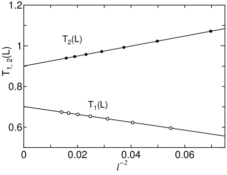
We plot as a function of with for the best fitted parameters in Fig. 1. We represent the temperature in units of . The error bars are smaller than the size of marks. Our estimate of is 0.8933(6); the number in the parentheses denotes the uncertainty in the last digits. We have estimated the uncertainty by the test of the data for 100 samples. This value is consistent with the estimates of recent studies; 0.89213(10) by the Monte Carlo simulation [10], and 0.894 by the short-time dynamics [11]. The constant , in Eq. (13), is estimated as =1.73(2).
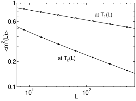
Let us consider the magnetization at to discuss the critical exponent . In Fig. 2, we plot as a function of in logarithmic scale. We expect the FSS of the form , but there are small corrections. The importance of the multiplicative logarithmic corrections were pointed out [4, 21]. Using the form
| (14) |
we obtain and . We show the fitting curve obtained by using Eq. (14) in Fig. 2. This value of is a little bit smaller than the theoretical prediction, 1/4 (=0.25). Our logarithmic-correction exponent is compatible with Janke’s result for thermodynamic data [21], but different from the theoretical prediction [4].
IV Clock model
Next turn to the -state clock model. Because of the reflection symmetry, we confine ourselves to the case of even . Then, the same procedure can be used as the XY model. One thing we should have in mind is that the axis of the vector should be chosen from one of directions in Eq. (1) or the middle of two of them. We plot the high-temperature transition temperature of the 6-state clock model as a function of in Fig. 3. The estimate of is 0.9008(6), which is more precise than the previous estimates; 0.92(1) [13] and 0.90 [14]. The plot of at as a function of for the 6-state clock model is given in Fig. 4. The estimate of is 0.243(5) by the analysis of the multiplicative logarithmic corrections, Eq. (14), and the exponent is estimated as 0.037(5).
For the second-order transition, the curves of the existence probability of different sizes cross at as far as the corrections to FSS are negligible; this is the same as the behavior of the Binder ratio [22]. For the KT transition, however, is not the crossing point but the spray-out point. Therefore, can be searched only from the high-temperature side, and only from the low-temperature side. The value of at is close to 1. In principle, we can use the same procedure as the study of ; we may change the setting value of , 1/2, to a higher one by introducing a biased random walk. However, it is difficult to resolve the size dependence for lower temperatures. Therefore, we employ a slightly different approach for the analysis of the phase transition at . When judging whether clusters are percolating or not, we consider another type of clusters. Instead of choosing the vector randomly in Eq. (3), we choose the vector as
| (15) |
with , or more generally we may choose such that
| (16) |
with some fixed angle . With this choice, the existence probability for the percolation of only (or ) Ising spins holds the same FSS property as the total . As a result, we can control the value of at so as to apply the FSS analysis easily with an appropriate .
The low-temperature transition temperature of the 6-state clock model obtained by the above modified approach is plotted as a function of also in Fig. 3. As the angle in Eq. (16), we have used . Our estimate of is 0.7014(11), which is more precise again than the previous estimates; 0.68(2) [13] and 0.75 [14]. The plot of at for the 6-state clock model is also given in Fig. 4. The estimate of is 0.113(3) by the analysis of the multiplicative logarithmic corrections, Eq. (14), and the exponent is estimated as 0.017(4). The previous estimates of are 0.100 [13] and 0.15 [14].
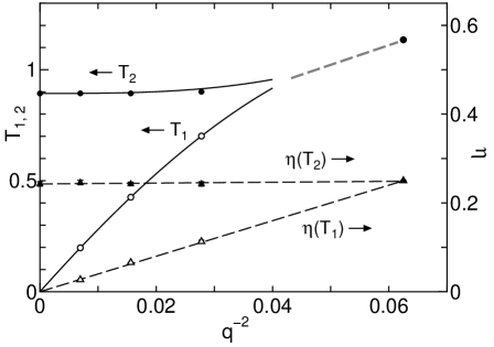
We have also made simulations for and . The estimates of the transition temperatures and those of and for =6, 8, 12, and (the XY model) are tabulated in Table I. The -dependence of transition temperatures and exponents are shown in Fig. 5. There, the exact results for are also given; that is, the Ising singularity at with . The transition temperature becomes smoothly lower with larger ; in the lowest order we find that , which is consistent with the theoretical prediction [5]. The critical exponent at is a universal constant, and compatible with the theoretical prediction . The estimates of the critical exponent at remarkably coincide with the theoretical prediction ; 1/9=0.111 for =6, 1/16=0.0625 for =8, and 1/36=0.0278 for =12. This is the first systematic report of confirming the theoretical prediction.
V Summary and discussions
To summarize, we have extended the PCC algorithm [17] to the study of the XY and clock models. Wolff’s idea of the embedded cluster formalism [16] is used for treating the system with the vector order parameter. The KT transitions of the 2D XY and clock models are studied by using the FSS analysis based on the KT form of the correlation length. For dealing with the low-temperature transition temperature, , we have employed a slightly modified algorithm. Investigating the clock models, we have systematically confirmed the prediction of . We have shown that small logarithmic corrections are present in the KT transitions. The sign of the logarithmic-correction exponent is positive for all cases of the XY model and the clock models at both and , which is compatible with Janke’s result [21], but different from the theoretical prediction [4]. The present precise numerical results may stimulate the refined renormalization-group study of the KT transitions.
In the previous numerical studies of the KT transitions, one might resort to a big scale calculation using an extensive computer resource [7], or one might use some special boundary conditions [10]. It is due to the subtlety of the KT phase transitions; that is, is not the crossing point but the spray-out point of the existence probability or the Binder parameter. Moreover, the low-temperature transition for the clock model is difficult to study because the system is nearly ordered; it is more difficult for larger . We should stress that using the present efficient method of numerical simulation, we have successfully made a systematic study of the XY and clock models with much less efforts.
Our formalism of the vector order parameter is easily extended to the general model, where the percolation of types of Ising spins will be considered. Then, more problems of interest can be studied by the PCC algorithm. The PCC algorithm can be also applied to the quantum Monte Carlo simulation with the cluster algorithm [23, 24]. It will be interesting to compare the present result with the quantum XY model.
Acknowledgments
We thank N. Kawashima, H. Otsuka, M. Itakura, and Y. Ozeki for valuable discussions. Thanks are also due to M. Creutz for bringing our attention to the clock model having two phase transitions. The computation in this work has been done using the facilities of the Supercomputer Center, Institute for Solid State Physics, University of Tokyo. This work was supported by a Grant-in-Aid for Scientific Research from the Japan Society for the Promotion of Science.
REFERENCES
- [1] Electronic address: ytomita@phys.metro-u.ac.jp
- [2] Electronic address: okabe@phys.metro-u.ac.jp
- [3] J. Kosterlitz and D. Thouless, J. Phys. C 6, 1181 (1973). See also V. L. Berezinskii, Zh. Eksp. Teor. Fiz. 59, 907 (1970) [Sov. Phys. JETP 32, 493 (1971)].
- [4] J. M. Kosterlitz, J. Phys. C 7, 1046 (1974).
- [5] J. V. José, L. P. Kadanoff, S. Kirkpatrick, and D. R. Nelson, Phys. Rev. B 16, 1217 (1977).
- [6] H. Weber and P. Minnhagen, Phys. Rev. B 37, 5986 (1988).
- [7] R. Gupta and C. F. Baillie, Phys. Rev. B 45, 2883 (1992).
- [8] H. Kawamura and M. Kikuchi, Phys. Rev. B 47, 1134 (1993).
- [9] P. Butera and M. Comi, Phys. Rev. B 47, 11969 (1993).
- [10] P. Olsson, Phys. Rev. B 52, 4526 (1995).
- [11] B. Zheng, M. Schulz, and S. Trimper, Phys. Rev. E 59, R1351 (1999).
- [12] S. G. Chung, Phys. Rev. B 60, 11761 (1999)
- [13] M. S. S. Challa and D. P. Landau, Phys. Rev. B 33, 437 (1986).
- [14] A. Yamagata and I. Ono, J. Phys. A 24, 265 (1991).
- [15] R. H. Swendsen and J. S. Wang, Phys. Rev. Lett. 58, 86 (1987).
- [16] U. Wolff, Phys. Rev. Lett. 62, 361 (1989).
- [17] Y. Tomita and Y. Okabe, Phys. Rev. Lett. 86, 572 (2001).
- [18] Y. Tomita and Y. Okabe, Phys. Rev. E 64, 036114 (2001).
- [19] P. W. Kasteleyn and C. M. Fortuin, J. Phys. Soc. Jpn. Suppl. 26, 11 (1969); C. M. Fortuin and P. W. Kasteleyn, Physica 57, 536 (1972).
- [20] J. Machta, Y. S. Choi, A. Lucke, T. Schweizer, and L. V. Chayes, Phys. Rev. Lett. 75, 2792 (1995).
- [21] W. Janke, Phys. Rev. B 55, 3580 (1997).
- [22] K. Binder, Z. Phys. B 43, 119 (1981).
- [23] H. G. Evertz, G. Lana, and M. Marcu, Phys. Rev. Lett. 70, 875 (1993).
- [24] N. Kawashima and J. E. Gubernatis, Phys. Rev. Lett. 73, 1295 (1994).


| 0.9008(6) | 0.243(4) | 0.7014(11) | 0.113(3) | |
| 0.8936(7) | 0.243(4) | 0.4259(4) | 0.0657(2) | |
| 0.8937(7) | 0.246(5) | 0.1978(5) | 0.0270(5) | |
| XY () | 0.8933(6) | 0.243(4) | ——— | ——— |