Yang-Lee zeros for a
nonequilibrium phase transition

Abstract

Equilibrium systems which exhibit a phase transition can be studied by investigating the complex zeros of the partition function. This method, pioneered by Yang and Lee, has been widely used in equilibrium statistical physics. We show that an analogous treatment is possible for a nonequilibrium phase transition into an absorbing state. By investigating the complex zeros of the survival probability of directed percolation processes we demonstrate that the zeros provide information about universal properties. Moreover we identify certain non-trivial points where the survival probability for bond percolation can be computed exactly.

1 Introduction

The investigation of nonequilibrium systems is of great importance since most phenomena in nature take place under nonequilibrium conditions. In this field, as in equilibrium physics, phase transitions are particularly interesting. However, when dealing with nonequilibrium systems one cannot utilize such a well-established theoretical framework as in equilibrium statistical mechanics. Therefore it is interesting to investigate which concepts of equilibrium physics can be transfered to nonequilibrium systems.

An important concept of equilibrium statistical physics is the theory of Yang and Lee [1] for the emergence of nonanalytic behaviour at phase transtitions. Only recently these ideas have been applied to an integrable nonequilibrium model [2]. In the present work we use similar techniques to investigate directed percolation (DP) [3] as a paradigm for nonintegrable systems far from equilibrium. We show that it is possible to transfer the ideas of Yang and Lee to DP and that this method does indeed provide information about universal properties of the phase transition.

1.1 Yang and Lee’s theory in equilibrium statistical physics

We shall shortly sketch the ideas of complex zeros of the partition function in equilibrium statistical mechanics. Taking the Ising model without an external magnetic field as an example, we consider a system of $N$ spins $s_{i}$ ($s_{i}=\pm 1,\,i=1,\ldots,N$) on a lattice where the spins interact with their nearest neighbours, denoted by $<i,j>$. The total energy ${\cal H}(\left\{s_{i}\right\})$ of a configuration $\left\{s_{i}\right\}$ of the spins is given by ${\cal H}(\left\{s_{i}\right\})=-J\sum_{<i,j>}s_{i}s_{j}$. The system is said to be in thermal equilibrium at temperature $T$ when the probability distribution $P(\left\{s_{i}\right\})$ to find the system in configuration $\left\{s_{i}\right\}$ is given by the stationary Gibbs ensemble $P(\left\{s_{i}\right\})\propto\rme^{-\beta{\cal H}(\left\{s_{i}\right\})},\ \beta=k_{\rm B}T$, where $k_{\rm B}$ is Boltzmann’s constant. In that case the statistical properties of the system are fully determined by the canonical partition function

$$Z_{N}(T) = \sum_{\left\{s_{i}\right\}}\rme^{-\beta{\cal H}(\left\{s_{i}\right\})}=\sum_{\left\{s_{i}\right\}}x^{r(\left\{s_{i}\right\})}\quad{\rm with}$$ (2)

$$x=\rme^{\beta J}>0\quad,\quad r(\left\{s_{i}\right\})=\sum_{<i,j>}s_{i}s_{j}\ .$$

For finite system size $Z_{N}$ can be expressed as the ratio of two polynomials in $x$ with integer coefficients. The free energy per lattice site is obtained from $Z_{N}$ through

$$f=\lim_{N\to\infty}\left(-\frac{1}{\beta N}\ln Z_{N}\right)$$ (3)

The hallmark of phase transitions is the appearance of nonanalyticities. Since in Equation (3) singularities occur as zeros of the partition function $Z_{N}$, these are good candidates for indicating a phase transition. However, $Z_{N}$ has no zeros for a positive real temperature so that there is no phase transition for finite $N$. This led Yang and Lee to study the complex zeros of $Z_{N}$, which in this case correspond to complex temperatures, and examine their behaviour as the system size grows. They argued that in the thermodynamic limit $N\to\infty$ in (3), if the model exhibits a phase transition, an ever increasing number of complex zeros accumulate in the vicinity of a point on the positive real axis, which corresponds to a physical temperature. The zeros thereby induce singularities at the critical point in the thermodynamic limit, thus explaining the crossover to nonanalyticity at the transition in the limit of an infinite system size. Such a behaviour has been observed for many equilibrium models. Moreover, several features of the distribution of zeros have been related to universal properties of the system under consideration [4].

1.2 Directed percolation, a process away from equilibrium

Since nonequilibrium systems do not obey the stationary Gibbs ensemble they cannot be handled using the partition function of equilibrium statistical physics. Instead they are described by the time-dependent probability distribution $P_{t}(\left\{s_{i}\right\})$ which has to be derived from the master equation. In most cases this cannot be done exactly. Nevertheless, the concept of universality, well-known from equilibrium statistical physics, proves to be suitable for nonequilibrium phase transitions as well. In this context models exhibiting a transition from a fluctuating active phase to a nonfluctuating inactive phase (absorbing state) have been extensively studied [5, 6, 7, 8]. These models are used to describe spreading processes as e.g. forest fires, where a spreading agent can either spread over the entire system or die out after some time. The two phases are seperated by a nonequilibrium phase transition. The most prominent universality class of transitions into an absorbing state is that of directed percolation. Directed percolation is an anisotropic variant of ordinary percolation in which activity can only percolate along a given direction in space. Regarding this direction as a temporal degree of freedom, DP can be interpreted as a dynamical process. Directed percolation emerges in a variety of physical problems ranging from catalytic reactions on surfaces [9] to spatio-temporal intermittency in magnetic fluids [10].

1.3 Realizations of DP

Simple realizations of DP are directed bond (DPb) and directed site percolation (DPs) on a tilted square lattice (see Figure 1). In directed bond percolation the bonds are conducting with probability $p$ and non-conducting with probability $1-p$. In this model sites at time $t>0$ are activated by directed paths of conducting bonds, originating from active sites at time $t=0$. A cluster consists of all sites that are connected by such paths of conducting bonds to active sites in the initial state. In directed site percolation on the other hand all bonds are conducting while the sites themselves can be either permeable ($p$) or blocked ($1-p$). Activity can spread from permeable site to permeable site. A cluster is formed by permeable sites that are connected to active sites at time $t=0$ by a directed path of bonds that only connect permeable sites.

The order parameter which characterizes the phase transition is the probability $P(\infty)$ that a randomly chosen site belongs to an infinite cluster. For $p>p_{\rm c}$ this probability is finite whereas it vanishes for $p\leq p_{\rm c}$. Close to the phase transition $P(\infty)$ is known to vanish algebraically as $P(\infty)\sim(p-p_{\rm c})^{\beta}$, where $\beta$ is an universal critical exponent. In addition, the DP process is characterized by a spatial correlation length $\xi_{\bot}$ (perpendicular to time) and a temporal correlation length $\xi_{||}$. As $p$ approaches $p_{\rm c}$ these length scales are known to diverge as

$$\xi_{\bot}\sim|p-p_{\rm c}|^{-\nu_{\bot}}\ ,\qquad\xi_{||}\sim|p-p_{\rm c}|^{-\nu_{||}}$$ (4)

with the critical exponents $\nu_{\bot}$ and $\nu_{||}$. The scaling behaviour (4) implies that DP is invariant under the scaling transformations

$$x\to\Lambda x\ ,\quad t\to\Lambda^{z}t\ ,\quad(p-p_{\rm c})\to\Lambda^{-1/\nu_{\bot}}(p-p_{\rm c})\ ,$$ (5)

where $x$ is the position and $z=\nu_{||}/\nu_{\bot}$ is the so-called dynamic exponent. Numerical estimates for the values of $p_{\rm c}$ and the critical exponents in 1+1 dimensions are $p_{\rm c}=0.6447001(1)$, $\beta=0.27649(4)$, $\nu_{\bot}=1.096844(14)$ and $\nu_{||}=1.733825(15)$ [11] (bond percolation) and $p_{\rm c}=0.705489(4)$ [12] (site percolation).

Although DP can be defined and easily simulated, it is one of the very few systems for which – even in one spatial dimension – no analytical solution is known, suggesting that DP is a non-integrable process. In fact, the values of the percolation threshold and the critical exponents are not simple numerical fractions but seem to be irrational instead.

Figure 1: Lattice geometry of DP on a tilted square lattice in 1+1 dimensions. In both cases (DPb and DPs) sites can be eiter active ($s_{j,t}=1$) or inactive ($s_{j,t}=0$). In DPb activity can percolate forward in time through bonds (solid lines) which are conducting. In DPs acitvity can percolate through bonds that connect permeable sites.

1.4 Yang and Lee zeros for directed percolation

To apply the idea of Yang-Lee zeros to DP, we consider the order parameter in a finite system as a function of the percolation probability $p$ in the complex plane. This can be done by studying the time-dependent survival probability $P(t)$, which is defined as the probability that a cluster generated in a single site at time $t=0$ survives up to time $t$ (or even longer). For a finite system $P(t)$ can be expressed as a polynomial in $p$ (see below). Note that $\lim_{t\to\infty}P(t)$ and the order parameter $P(\infty)$ coincide.

The survival probability and the partition function (2) show a similar behaviour in many respects. For finite systems $P(t)$ and $Z_{N}$ do not have relevant zeros in the physical region of the control parameter $0\leq p\leq 1$ and $0<T<\infty$ although the phase transition is marked by a vanishing $P(t)$ and $Z_{N}$ at the critical points in the limit of infinite systems. At those points both functions exhibit nonanalytic behaviour. The zeros of $P(t)$ and $Z_{N}$ are generated by polynomials with real integer coefficients, thus the zeros come in complex-conjugate pairs.

According to Yang and Lee the increasing system size is accompanied by an approach of some of the complex zeros of $Z_{N}$ to the physical region of the control parameter, while the accumulation point marks the critical point. We show that the complex zeros of $P(t)$ approach the critical value $p_{\rm c}$ on ’trajectories’ for increasing time $t$ and that the distance between the zeros and the critical point is related to the critical exponent for the temporal correlation length.

1.5 Determining the survival probability

In directed bond (site) percolation the survival probability $P(t)$ is given by the sum over the weights of all possible configurations of bonds (sites) for which the process survives at least up to time $t$. Each conducting bond (permeable site) contributes to the weight with a factor $p$, while each non-conducting bond (blocked site) contributes with a factor $1-p$. However, the states of those bonds (sites) which do not touch the actual cluster are irrelevant as they do not contribute to the survival of the cluster. Therefore, it is sufficient to consider the sum over all possible clusters $\cal C$ of bonds (sites) connected to the origin. Each cluster is weighted by the contributions of the conducting bonds (permeable sites) belonging to the cluster and the non-conducting bonds (blocked sites) belonging to its hull. Roughly speaking, the hull surrounds the cluster. More precisely the hull of a cluster is the set of non-conducting bonds (blocked sites) that would contribute to the cluster if they were conducting (permeable) (see Figure 2). Thus the survival probability can be expressed as

$$P(t)=\sum_{\cal C}p^{n}(1-p)^{m}\,,$$ (6)

where the sum runs over all clusters reaching the horizontal row at time $t$. For each cluster $n$ denotes the number of its bonds (sites), while $m$ is the number of bonds (sites) belonging to its hull. Note that in this sense the hull does not include bonds connecting sites at time $t$ and $t+1$ (DPb) or sites at time $t+1$ (DPs) since the cluster may survive even longer. Summing up all weights in Equation (6) one obtains a polynomial. As can be verified, the first few polynomials for the survival probability in the directed bond percolation process are

Figure 2: Example of clusters which survive until time $t=3$. Acitve sites are shown as black circles, conducting bonds as solid lines. Left: Dashed lines denote the hull, irrelevant bonds are not shown. The corresponding weight to the survival probability $P(3)$ in (6) is $p^{4}(1-p)^{4}$. Right: White patterned circles belong to the hull. Simple white circles are irrelevant for the survival of the cluster. The corresponding weight to $P(3)$ is $p^{4}(1-p)^{3}$.

$$P(0)=1$$ (7)

$$P(1)=2p-p^{2}$$

$$P(2)=4p^{2}-2p^{3}-4p^{4}+4p^{5}-p^{6}$$

$$P(3)=8p^{3}-4p^{4}-10p^{5}-3p^{6}+18p^{7}+5p^{8}-30p^{9}+24p^{10}-8p^{11}+p^{12}$$

$$P(4)=16p^{4}-8p^{5}-24p^{6}-8p^{7}+6p^{8}+84p^{9}-29p^{10}-62p^{11}-120p^{12}$$

$$\qquad\quad+244p^{13}+75p^{14}-470p^{15}+495p^{16}-268p^{17}+83p^{18}-14p^{19}+p^{20}\,.$$

As $t$ increases the number of cluster configurations grows rapidly, leading to complicated polynomials with very large coefficients (e.g. for $t=15$ the largest coefficient for bond percolation is of order $10^{44}$).

The paper is structured as follows. In Section 2 we investigate if the distribution of zeros is totally dependent on microscopic details of the underlying model or whether it also contains universal features. We ask whether the distribution is related to some of the critical exponents which characterize the phase transition of directed percolation. Section 3 presents certain non-trivial points where the polynomials $P(t)$ for bond percolation can be calculated exactly for all times. Section 4 ends with a conclusion. In A we show that the value of the survival probability can be computed by Monte Carlo simulations even if $p$ is a complex number. The first coefficients of the polynomials $P(t)$ for bond percolation are discussed in B.

2 Universal properties

The distribution of the zeros of $P(t)$ (from $t=8$ to $t=15$) in the neighbourhood of the critical point is shown in Figure 3.

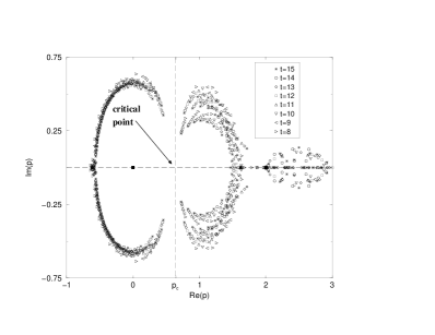
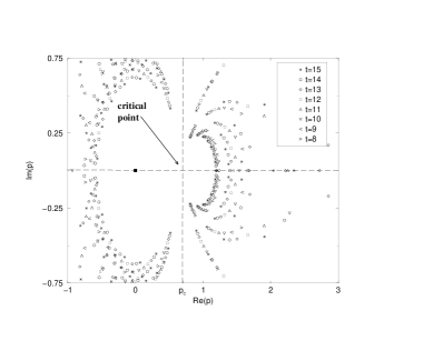
Figure 3: Zeros of the survival probability $P(t)$ in the complex plane.
Left: Directed bond percolation. Right: Directed site percolation.

Away from the critical point the appearance of the distributions for DPb and DPs is quite different. This implies that in this region the distribution of zeros depends strongly on microscopic details and hence is non-universal. However, there is also a general feature which can be observed in both cases. The innermost zeros approach the critical point on ‘trajectories’ as $t$ increases (see Figure 4).

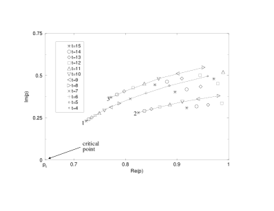
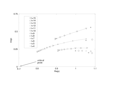
Figure 4: Zeros approaching the critical point. Three ‘trajectories’ are enumerated and shown as dashed lines. Left: Directed bond percolation. Right: Directed site percolation.

We applied a standard Bulirsch-Stoer (BST) acceleration algorithm [13] to the set of zeros of each enumerated ‘trajectory’ of Figure 4 to determine $\lim_{t\rightarrow\infty}{\rm Re}\left(p^{\rm zero}(t)\right)$ and $\lim_{t\rightarrow\infty}{\rm Im}\left(p^{\rm zero}(t)\right)$. The results are listed in Table 1.

trajectory	${\rm Re}\left(p^{\rm zero}_{t\to\infty}\right)$	${\rm Im}\left(p^{\rm zero}_{t\to\infty}\right)$	trajectory	${\rm Re}\left(p^{\rm zero}_{t\to\infty}\right)$	${\rm Im}\left(p^{\rm zero}_{t\to\infty}\right)$
bond 1	0.64472(1)	0.0001(1)	site 1	0.70547(3)	0.0001(3)
bond 2	0.6445(2)	0.008(1)	site 2	0.709(4)	0.006(1)
bond 3	0.6470(4)	0.051(7)	site 3	0.712(1)	0.01(1)

Table 1: Bulirsch-Stoer extrapolants for the zeros of the ‘trajectories’ from Figure 4 for both bond and site percolation in 1+1 dimensions.

Although we calculated the zeros only for small systems (until $t=15$) the extrapolants accord fairly well with the numerical values of the percolation threshold $p_{\rm c}=0.6447001(1)$ (bond percolation) and $p_{\rm c}=0.705489(4)$ (site percolation). Thus a similar scenario as observed by Yang and Lee for equilibrium phase transitions proves to be suitable for the nonequilibrium phase transition of DP. As time increases the zeros of the survival probability $P(t)$ approach the real axis between $p=0$ and $p=1$. The accumulation point is the critical point.

So far we have shown that the zeros of $P(t)$ provide information about the existence of the phase transition and about the critical value $p_{\rm c}$. However, the value of $p_{\rm c}$ is non-universal and depends on the particular realization of DP. On the contrary universal features are independent of the microscopic details of the underlying process. On each ‘trajectory’ of Figure 4 we calculated the distance between the zeros and the critical point $d(t)=|p^{\rm zero}(t)-p_{c}|$ with the values of $p_{\rm c}$ as given in section 1.3. According to Equation (4) and simple scaling arguments we expect $d(t)$ to decrease as $d(t)\sim t^{-1/\nu_{||}}$. Application of the BST algorithm yields results which support this claim, as shown in Table 2.

trajectory	$1/\nu_{||}$	trajectory	$1/\nu_{||}$
bond 1	0.57675(3)	site 1	0.5765(7)
bond 2	0.575(2)	site 2	0.5771(2)
bond 3	0.576(4)	site 3	0.5731(2)

Table 2: Bulirsch-Stoer extrapolants for the exponent $1/\nu_{||}$. On each ‘trajectory’ in Figure 4 the distance $d(t)=|p^{\rm zero}(t)-p_{c}|$ is assumed to decrease as $d(t)\sim t^{-1/\nu_{||}}$.

The extrapolants are in fairly good agreement with the numerical value of $1/\nu_{||}=0.57676$, even for small systems. This means that universal properties of the phase transition of directed percolation are encoded in the complex zeros of the survival probability $P(t)$. Figure 5 shows the used data and the asymptotic power law $d(t)\sim t^{-1/\nu_{||}}$ with the numerical value of $\nu_{||}$.

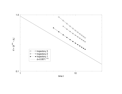
Figure 5: The distance from the critical point $d=|p^{\rm zero}-p_{\rm c}|$ versus time $t$. For comparison the power law $d\sim t^{-1/\nu_{||}}$ is shown, with $\nu_{||}=1.7338$. Left: Directed bond percolation. Right: Directed site percolation.

3 Exact results

In this section we will address a particularly surprising observation, namely the existence of certain points on the real axis where the polynomials $P(t)$ for bond percolation can be solved exactly for all values of $t$. Beside the trivial points $p=0$ (where $P(t)=\delta_{t,0}$) and $p=1$ (where $P(t)=1$) we find a $t$-independent zero at $p=2$ and, even more surprisingly, a very simple solution if $p$ is equal to one of the Golden Ratios $(1\pm\sqrt{5})/2$. The Golden Ratios are the roots of the quadratic equation $p^{2}=p+1$ and play an important role not only in number theory [15] but also in other fields ranging from chaotic systems [16] to arts [17]. Although these special points are located outside the physically accessible region $0\leq p\leq 1$, their existence may be helpful for further investigations of the polynomials $P(t)$.

3.1 Time-independent zero at $p=2$

For $p=2$ and $t\geq 1$ all polynomials $P(t)$ vanish identically. This can be shown as follows. Let us consider the probability $R(t)$ that a cluster dies out at time $t$, i.e., the row at time $t$ is the last row reached by a cluster. Obviously $R(t)$ is related to the survival probability by

$$R(t)=P(t)-P(t+1)\,.$$ (8)

Clearly, $R(t)$ can be expressed as a weighted sum over the same set of clusters as in (6). However, in the present case the weights differ from those in Equation (6) by the number of non-conducting bonds in the clusters hull between $t$ and $t+1$ since it is now required that all sites at time t+1 are inactive (see Figure 6). This means that $R(t)$ can be expressed as

$$R(t)=\sum_{\cal C}p^{n}(1-p)^{m}(1-p)^{2k}\,,$$ (9)

where $n$, $m$ and ${\cal C}$ have the same meaning as in (6) and $k$ is the number of active sites in the horizontal row at time $t$. Obviously, for $p=2$ the additional factor $(1-p)^{2k}$ drops out so that $P(t)=R(t)$ for all values of $t$. Moreover, $R(0)=P(0)=1$ (for $p=2$). Combining these results with Equation (8) we arrive at $P(t)=0$ for $t>0$, which completes the proof.

Figure 6: Example for different weights for $P(t)$ and $R(t)$. Left: The contribution of the shown cluster to $P(3)$ in (6) is $p^{4}(1-p)^{2}$. Right: The contribution of the cluster to $R(3)$ in (9) is $p^{4}(1-p)^{6}$ since it is required that active sites at $t=3$ are not connected to sites at $t=4$ by active bonds.

3.2 Exact solution for $p$ at the Golden Ratio

For $p=(1\pm\sqrt{5})/2$ we find that the survival probability ‘oscillates’ between two different values, namely

$$P(t)=\cases{1&if $t$ is even\\ \frac{\pm\sqrt{5}-1}{2}&if $t$ is odd.\\ }$$ (10)

Figure 7: Decomposition of the configurational sum of non-surviving clusters into three subsets. Open and closed bonds are denoted by solid (dashed) lines. Bonds which are not shown may be either open or closed. The box includes all bonds contributing to the factor $\hat{Q}_{1}$ while all other bonds contribute to the factor $\hat{Q}_{2}$. The proof shows that the configurations in (a) and (b) cancel each other so that only the configurations of (c) contribute to $Q$. Iterating the procedure by shifting the box to the right, it can be shown that all sites at $t-2$ and $t-1$ have to be zero.

To prove this result, we first verify that (10) is indeed satisfied for $t=0$ and $t=1$. Then we show that

$$P(t)=P(t-2)\qquad\mbox{for }t\geq 2\quad\mbox{and}\quad p=(1\pm\sqrt{5})/2\,.$$ (11)

However, instead of analyzing the survival probability directly, it turns out to be more convenient to consider the complementary probability $Q(t)=1-P(t)$ that a cluster does not survive until time $t$. Obviously, $Q(t)$ is the sum over the weights of all clusters which do not reach the horizontal row at time $t$, i.e., we impose the boundary condition $s_{0,t}=s_{1,t}=\ldots=s_{t,t}=0$. Depending on the states of the two sites $s_{0,t-1}$ and $s_{0,t-2}$ at the left edge of the clusters, this set of clusters may be separated into three different subsets, namely,

(a) a subset where $s_{0,t-1}=s_{0,t-2}=1$,

(b) a subset where $s_{0,t-1}=0$ and $s_{0,t-2}=1$, and

(c) a subset where $s_{0,t-1}=s_{0,t-2}=0$.

Next we show that the weights of the clusters in the subsets (a) and (b) cancel each other. To this end we note that the weighted sum $\hat{Q}(t)$ over all clusters in subsets $(a)$ and $(b)$ may be decomposed into two independent factors $\hat{Q}(t)=\hat{Q}_{1}\hat{Q}_{2}$, where $\hat{Q}_{1}$ depends only on the state of the three bonds between the sites $s_{0,t-2}$, $s_{0,t-1}$, $s_{0,t}$, and $s_{1,t}$ (inside the box in Figure 7), while $\hat{Q}_{2}$ accounts for all other relevant bonds. Obviously, the first factor is given by

$$\hat{Q}_{1}^{(a)}=p(1-p)^{2}\,,\qquad\hat{Q}_{1}^{(b)}=1-p\,,$$ (12)

while $\hat{Q}_{2}$ takes the same value in both subsets. Thus, if $p$ is given by the Golden Ratio, we obtain $\hat{Q}_{1}^{(a)}+\hat{Q}_{1}^{(b)}=\hat{Q}_{1}(t)=0$ and therefore the weights of subsets (a) and (b) cancel each other. Consequently, all remaining contributions to $Q(t)$ come from the clusters in subset (c) where the sites $s_{0,t-1}$ and $s_{0,t-2}$ are inactive. Now we can iterate this procedure by successively considering the sites $s_{j,t-1}$ and $s_{j,t-2}$ from the left to the right, where $j=1\ldots t-2$. In this way it can be shown that all these sites have to be inactive as well. Therefore, the only surviving contributions are those in which the entire row of sites at $t-2$ is inactive, implying that $Q(t)=Q(t-2)$. The proof of Equation (10) then follows by induction.

4 Conclusions

In this paper we have investigated the applicability of Yang-Lee theory to the nonequilibrium phase transition of directed percolation. In Section 1 we developed an idea of how to transfer the concepts of Yang and Lee to the phase transition of DP by studying the complex zeros of the survival probability. In Section 2 we showed that a similar scenario as observed for equilibrium phase transitions is also suitable for DP, namely complex zeros approaching the critical point for increasing system size. Moreover, we could extract the value of the critical exponent for the temporal correlation length from the distribution of zeros. Hence the zeros encode univerals properties of the phase transition of DP. Section 3 presented exact results on the survival probability of bond percolation which may be helpful for further investigations. More precisely, we proved that there are certain non-trivial values of $p$ for which the values of the polynomials $P(t)$ can be calculated exactly for all times.

Appendix A MC-Simulations

Here we demonstrate that the value of the survival probability for a complex percolation probability $p$ as well as the polynomials $P(t)$ are accessible by computer simulations.

Let us consider the definition of the survival probability as a sum over configurations of surviving clusters in Equation (6). Formally this expression can be rewritten as

$$P(t)=\sum_{\cal C}p^{n}(1-p)^{m}=\sum_{\cal C}q^{n}(1-q)^{m}\,\underbrace{\frac{p^{n}(1-p)^{m}}{q^{n}(1-q)^{m}}}_{f_{n,m}}$$ (13)

where $n$ and $m$ denote the number of bonds of the cluster and of its hull respectively. Therefore, instead of simulating the system at a given $p$, we may simulate it using a different percolation probability $q$ reweighting each cluster by the factor $f_{n,m}$. While $q\in(0,1)$ still has to be a real number, $p$ is no longer restricted to be real, it can be any complex number. Using this reweighting technique it is in principle possible to access the entire complex plane by numerical simulations. For any finite $t$ such a simulation is stable and will converge to the correct result. But even for small $t$ the convergence time can be very long, limiting the range of applications.

Using the reweighting technique it is also possible to approximate the coefficients of the polynomial $P(t)=\sum_{k}a_{k}p^{k}$ by considering $p$ as a free parameter and expanding the term $(1-p)^{m}$ in Equation (13). The coefficients are then given by

$$a_{k}=\sum_{\cal C}\,q^{n}(1-q)^{m}\,\frac{C(m,k-n)(-1)^{k-n}}{q^{n}(1-q)^{m}}\,,$$ (14)

where $q\in(0,1)$ is again a free parameter and

$$C(m,k-n)=\left\{\begin{array}[]{cc}\frac{m!}{(k-n)!(m-k-n)!}&\mbox{ if }0\leq k-n\leq m\\ 0&\mbox{ otherwise }.\end{array}\right.$$ (15)

However, in most cases the direct construction of the polynomials using symbolic algebra turns out to be more efficient.

Appendix B First coefficients of the polynomials $P(t)$ in the limit $t\to\infty$

As can be seen in Equation (7) the first non-vanishing coefficient of the polynomial for the survival probability $P(t)=\sum_{n}a_{n}p^{n}$ for DPb is always a power of $2$. This contribution corresponds to the configurational weight of a surviving path without branches. The purpose of this appendix is to point out that even the following coefficients can be computed exactly, provived that $t$ is large enough. More specifically, we conjecture that

$$a_{t+k}=2^{t-k-1}\,q_{k}(t)\,,$$ (16)

where

$$q_{k}(t)=\sum_{m=0}^{M}b_{m}^{(k)}t^{m}\,,\qquad M=\left\{\begin{array}[]{ll}k/2&\mbox{ if }k\mbox{ even}\\ (k-1)/2&\mbox{ if }k\mbox{ odd}\end{array}\right.$$ (17)

is a finite polynomial in $t$. Using the explicit expressions for $P(t)$ up to $t=15$ we find that the first eight polynomials read

$$q_{0}(t) = 2$$

$$q_{1}(t) = -2$$

$$q_{2}(t) = -4-2t$$

$$q_{3}(t) = -2t$$

$$q_{4}(t) = -16+3t+t^{2}$$ (18)

$$q_{5}(t) = 32+t+3t^{2}$$

$$q_{6}(t) = -232+\frac{64}{3}t+3t^{2}-\frac{1}{3}t^{3}$$

$$q_{7}(t) = 808-\frac{34}{3}+5t^{2}-\frac{5}{3}t^{3}$$

We conjecture that the leading coefficient of these polynomials is given by

$$b_{M}^{(k)}=\left\{\begin{array}[]{ll}2(-1)^{M}/M!&\mbox{ if }k\mbox{ even }\\ 2(k-1)(-1)^{M}/M!&\mbox{ if }k\mbox{ odd }.\end{array}\right.$$ (19)

This implies that the first non-vanishing coefficients of the polynomial $P(t)$ grow in such a way that their limit $\lim_{t\to\infty}\frac{a_{t+k}}{2^{t}t^{M}}$ for fixed $k$ is well-defined. Summing up these contributions we obtain for the survival probability

$$P(t) \simeq (2p)^{t}\sum_{j=0}^{\infty}\frac{(-p^{2}t/4)^{j}}{j!}\,\Bigl{(}1+p(j-1/2)\Bigr{)}$$

$$= \frac{1}{4}(2p)^{t}e^{-p^{2}t/4}(4-2p-p^{3}t)\ .$$

Physically this expression corresponds to loop-free graphs and serves as an approximation close to $p=0$. The convergence radius of Equation (B) determined from $2p=e^{p^{2}/4}$ is $|p|<0.53744$. Note that none of the non-trivial roots computed up to $t=15$ lies inside this radius. We conjecture that this might be true for any $t$.

References

References

- [1] Yang C N and Lee T D (1952) Phys. Rev. 78 404; Lee T D and Yang C N (1952) Phys. Rev. 87 410
- [2] Arndt P F (2000) Phys. Rev. Lett. 84 814
- [3] Arndt P F, Dahmen S R and Hinrichsen H (2001) Physica A 295 128
- [4] Alves N A, Drugowich de Felicio J R and Hansmann U H E (2000) J. Phys. A 33 7489; Alves N A, Drugowich de Felicio J R and Hansmann U H E (1997) Inter. J. Mod. Phys. C 8 1063
- [5] Kinzel W (1983) Annals of the Israel Physical Society vol 5, ed. by Deutscher G, Zallen R and Adler J (Bristol: Adam Hilger)
- [6] Marro J and Dickman R (1999) Nonequilibrium phase transitions in lattice models (Cambridge: Cambridge University Press)
- [7] Hinrichsen H (2000) Adv. Phys. 49 815
- [8] Hinrichsen H (2000) Braz. J. Phys. 30 69
- [9] Voigt C A and Ziff R M (1997) Phys. Rev. E 56 R6241
- [10] Rupp P, Richter R and Rehberg I, cond-mat/0201308
- [11] Jensen I (1996) Phys. Rev. Lett.77 4988
- [12] Tretyakov A Y and Inui N (1995) J. Phys. A 28 3985
- [13] Henkel M and Schütz G (1988) J. Phys. A 21 2617
- [14] Derrida B, De Seze L and Itzykson C (1983) J. Stat. Phys. 33 559
- [15] see e.g.: Schroeder M (1999) Number Theory in Science and Communication (Springer Series in Information Science, vol. 7, Springer Verlag); Vajda S (1989) Fibonacci and Lucas numbers, and the Golden Section (Chichester: Horwood)
- [16] Ozorio de Almeida A M (1988) Hamiltonian Systems: Chaos and Quantization (Cambridge: Cambridge University Press)
- [17] Ghyka M (1977) The Geometry of Art and Life (New York: Dover Publications)