Anomalous Response Variability in a Balanced Cortical Network Model

Abstract

We use mean field theory to study the response properties of a simple randomly-connected model cortical network of leaky integrate-and-fire neurons with balanced excitation and inhibition. The formulation permits arbitrary temporal variation of the input to the network and takes exact account of temporal firing correlations. We find that neuronal firing statistics depend sensitively on the firing threshold. In particular, spike count variances can be either significantly greater than or significantly less than those for a Poisson process. These findings may help in understanding the variability observed experimentally in cortical neuronal responses.

1 Introduction

Cortical neuronal responses often exhibit a puzzling variability (see, e.g., [1]): spike count distributions obtained for repeated presentations of a stimulus are frequently broader than Poisson distributions with the same mean counts. In this paper we study the statistics of neuronal responses in a simple model network with balanced excitation and inhibition and find that they also show large variability. We focus on the so-called Fano factor $F$: the ratio of the variance of the spike count to its mean. It is equal to 1 for any Poisson process, homogeneous or inhomgeneous. We find that in our model it depends sensitively on the neuronal firing threshold: $F<1$ for high thresholds and $F>1$ for low ones, while mean spike counts are hardly affected by changes in threshold.

To study the responses in our model, we utilize mean field theory, which is exact in the limit of a large network with homogeneous connection probabilities [3]. It allows us to reduce the full network problem to one of a single neuron subject to a Gaussian synaptic current, the mean and covariance of which are self-consistently related to those characterizing the the neuron’s firing. It is Gaussian because of the central limit theorem: it is the sum of a large number of (what can be proved to be) independent contributions from the other neurons.

The mean field theory of balanced cortical networks has been studied by a number of authors [4, 5, 6, 7], but generally in or near steady firing states and assuming that the self-consistent current input is uncorrelated. Here, like ref. [3], we consider time-dependent external drive (as in an experimental trial) and color the noise correctly.

2 The Model

For these exploratory investigations, we use a network of $N$ mutually inhibitory neurons with a 10% connection probability. This is probably the simplest model for which one can achieve balanced asynchronous activity. The nonzero connections are of equal strength, and the synaptic currents are assumed to act instantaneously, i.e., each presynaptic spike depresses the postsynaptic potential discontinously by a fixed amount. We do not include transmission delays. This and other features, such as the presence of two neuronal populations, inhibitory and excitatory, can easily be incorporated into the model. A modest extension of this form might serve as a serious model of a cortical (mini)column. However, we believe that the basic dynamical features of balanced asynchronous networks are already captured in our simple all-inhibitory model.

We find it convenient to scale variables in the way used by van Vreeswijk and Sompolinsky [6]: When the mean number of neurons presynaptic to a given one is $K\gg 1$, each synaptic strength is given a value $J/\sqrt{K}$. Then the average synaptic current scales like $K\times 1/\sqrt{K}=\sqrt{K}$. It is inhibitory and is counterbalanced by an external excitatory current which is also proportional to $\sqrt{K}$. The fluctuations in the synaptic current are smaller than the mean by a factor of order $1/\sqrt{K}$, i.e., of order 1. In steady state, the two currents nearly cancel, leaving a net current of order 1. If the steady-firing state is stable, disturbances of the rates relax very rapidly, in a time of order $1/\sqrt{K}$. While this picture is something of a caricature, we believe it has some relevance to cortical dynamics.

Mean field theory can be used for any kind of neuron, but here we use leaky integrate-and-fire neurons. Thus, the (subthreshold) membrane potentials are described by

$$\dot{u}_{i}(t)=-\frac{1}{\tau}u_{i}+\sqrt{K}I^{0}_{i}(t)-\frac{J}{\sqrt{K}}\sum_{k,s}c_{ij}\delta(t-t^{s}_{j}),$$ (1)

where $\tau$ is their (common) membrane time constant, $I^{0}_{i}(t)$ is the excitatory external input current felt by neuron $i$, $c_{ij}$ is 1 or 0 according to whether there is a connection from neuron $j$ to neuron $i$, and $t^{s}_{j}$ is the $s$-th spike time of neuron $j$. The external input $I^{0}_{i}(t)$ represents input from elsewhere in the brain (e.g., the preceding stage in a sensory pathway), and as such is noisy itself. However, as the recurrent connections in the randomly-diluted network generate dynamical noise on their own, this extrinsic noise does not have a big qualitative effect, so we take $I^{0}_{i}(t)$ to be constant here. We also take it to be uniform across the population.

3 Mean Field Theory

As indicated above, in mean field theory, one studies a single neuron for which the recurrent synaptic current (the last term in (1)) is replaced by a self-consistent Gaussian current with self-consistent mean and variance. Explicitly, the subthreshold membrane potential of this single neuron obeys

$$\dot{u}=-\frac{1}{\tau}u_{i}+\sqrt{K}[I^{0}+I^{1}(t)].$$ (2)

Whenever $u$ reaches a threshold $\theta$, it fires a spike and $u$ is reset to zero. The effective recurrent current $I^{1}(t)$ has a mean

$$\langle I^{1}(t)\rangle=-Jr(t)$$ (3)

proportional to the instantaneous firing rate $r(t)$ of the neuron and a covariance

$$\langle\delta I^{1}(t)\delta I^{1}(t^{\prime})\rangle=\frac{1-K/N}{K}C(t,t^{\prime}),$$ (4)

where $C(t,t^{\prime})=\langle[S(t)-r(t)][S(t^{\prime})-r(t^{\prime})]\rangle$ is the autocorrelation funtion of the neuronal firing $S(t)=\sum_{s}\delta(t-t^{s})$. The $K$ in the denominator in (4) comes from the averaging over $K$ independent inputs, and the $1-K/N$ in the numerator is a correction for finite connection concentration $K/N$. It can be derived using the methods of ref. [8].

This model can not be solved exactly analytically, but it is simple to solve numerically, using the method first introduced for spin glasses by Eisfeller and Opper [9]. We start with a guess at the form of the mean and covariance function of the random current $I^{1}(t)$ and run a series of “trials”, in each of which we integrate (2) for an independent realization of $I^{1}(t)$. By averaging the output of the neuron over the trials, we get an estimate of $r(t)$ and $C(t,t^{\prime})$, which is used to generate new examples of $I^{1}(t)$ for another set of trials. This loop is then iterated until the statistics converge to self-consistency. In our calculations here, we used 10000 trials per iteration and up to 30 iterations.

Each trial was 100 integration steps (which we call “milliseconds”) long. We chose parameters $K=500$, $N=5000$, and $\tau=10$ ms. The external excitatory input $I^{0}(t)$ was constant at a low value (evoking a background firing rate of 3 Hz) during the first and last 10 ms. In the middle 80 ms, an additional “stimulus” input, which peaked about 15 ms after onset, was added. It typically evoked about 4-5 spikes, with peak rates around 100 Hz. The spike count distributions, PSTHs and covariance functions were computed for a number of values of the firing threshold $\theta$.

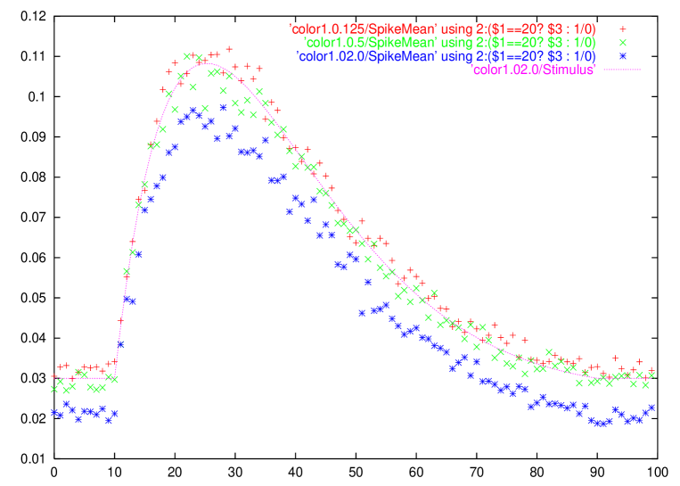
Figure 1: Stimulus (solid line) and PSTHs for three threshold values: 0.125 (red), 0.5 (green) and 2.0 (blue).

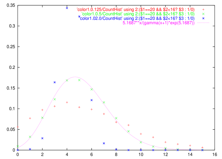
Figure 2: Count statistics for threshold 0.125 (red), 0.5 (green) and 2.0 (blue). The solid line shows the good fit to a Poisson distribution for the mean spike count (5.1687) obtained for threshold 0.5.

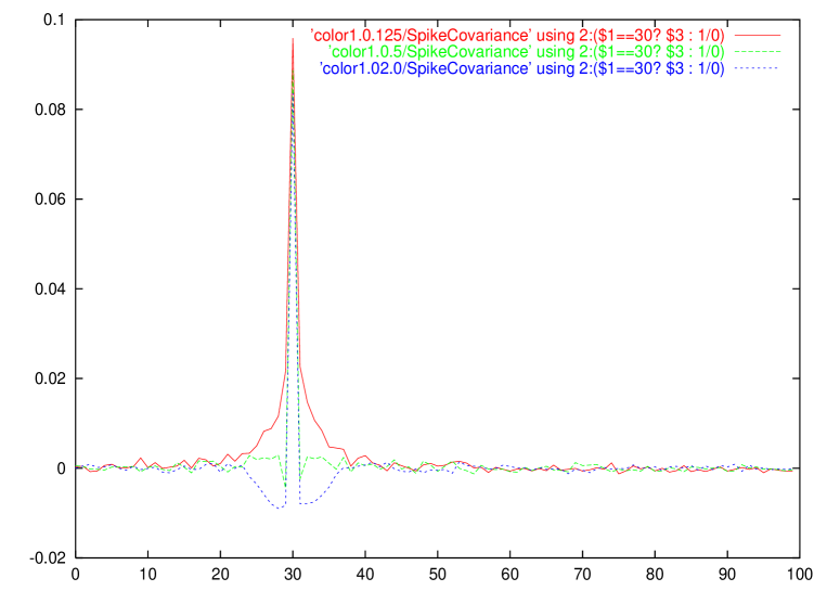
Figure 3: Autocorrelation functions $C(30,t^{\prime})$ for thresholds 0.125 (red), 0.5 (green) and 2.0 (blue).

4 Results

For all cases studied, the relaxation of the network to its state of balanced excitation and inhibition was very rapid, as expected, so the response tracked the time course of the excitatory external input closely (Fig. 1). The overall response strengths vary only weakly with threshold: a factor of 16 difference between the smallest and largest threshold values produced only a 20% difference in mean response. This is because the increased firing that would be produced by lowering the threshold is largely compensated by the comcomitant increase in inhibition.

However, varying the threshold had a strong effect on the irregularity of the firing. Fig. 2 shows the spike count distributions for three threshold values with ratio 1:4:16. While the intermediate value fits a Poisson distribution well, the low threshold leads to an anomalously broad distribution ($F=2.4$) and the high one to an anomalously narrow one ($F=0.25$).

These differences are also evident in the autocorrelation function $C(t,t^{\prime})$. Fig. 3) shows $C(t,t^{\prime})$ as a function of $t^{\prime}$ for a fixed value of $t$ for the same three threshold values as in the preceding figures. For the lowest threshold, there is a “hill” centered around $t=t^{\prime}$, while for the highest there is a valley. These are indicative of spike “bunching” and “antibunching”, respectively, leading naturally to the higher and lower spike count fluctuations seen in Fig. 2. The intermediate threshold value shows very little correlation (apart from the delta-function peak at $t=t^{\prime}$), consistent with the nearly-Poisson count distribution found in this case.

5 Discussion

Measured Fano factors in visual and IT cortex [1] vary over a range at least as large as the one-order-of-magnitude difference between those for the smallest and largest thresholds described above. Of course, threshold differences are not the only possible source of such response variability. We have also explored the effects of varying synaptic strengths, with similar results, and it seems likely that diffferences in a wide variety of single-neuron properties can have the same kind of effect.

Neurons in a local cortical network can not all be expected to have the same threshold, and, furthermore, their thresholds (or other parameters) may fluctuate (uncontrollably) from trial to trial. We have also found large variations in the Fano factor in a model where these fluctuations are assumed independent for different neurons and in different trials.

All these results are only suggestive, and more systematic work, both experiments and modeling, is called for. However, they do point to the possibility that the observed response variability of cortical neurons may be accounted for in terms of natural variations in properties from neuron to neuron and trial to trial.

References

- [1] E D Gershon, M C Wiener, P E Latham and B J Richmond, J Neurophysiol 79:1135-1144 (1998).
- [2] M C Wiener, M W Oram, Z Liu and B J Richmond, J Neurosci 21:8210-8221 (2001).
- [3] C Fulvi Mari, Phys Rev Lett 85:210-213 (2000).
- [4] D J Amit and N Brunel, Cerebral Cortex 7:237-252 (1997).
- [5] N Brunel, J Comput Neurosci 8:183-208 (2000).
- [6] C van Vreeswijk and H Sompolinsky, Science 274 1724-1726 (1996), Neural Comp 10:1321-1371 (1998).
- [7] P E Latham, B J Richmond, P G Nelson and S Nirenberg, J Neurophysiol 83:808-827 (2000).
- [8] R Kree and A Zippelius, Phys Rev A 36:4421-4427 (1987).
- [9] H Eisfeller and M Opper, Phys Rev Lett 68:2094-2097 (1992)