Microcanonical mean-field thermodynamics of self-gravitating and rotating systems

Abstract

We derive the global phase diagram of a self-gravitating $N$-body system enclosed in a finite three-dimensional spherical volume $V$ as a function of total energy and angular momentum, employing a microcanonical mean-field approach. At low angular momenta (i.e. for slowly rotating systems) the known collapse from a gas cloud to a single dense cluster is recovered. At high angular momenta, instead, rotational symmetry can be spontaneously broken and rotationally asymmetric structures (double clusters) appear.

The statistical equilibrium properties of systems of particles interacting via long-range forces (the so-called non-extensive systems) are currently the subject of intense research, both for their highly non-trivial thermodynamics (displaying such features as negative heat capacities thirring70 ; gross174 ) and for the considerable conceptual and technical difficulties they present. It is known that the long-range nature of the potential makes the canonical ensemble inadequate for describing their statics landau96 ; gallavotti99 ; padmanabhan90 , because the usual thermodynamic limit, where (number of particles) $N\to\infty$ and (volume) $V\to\infty$ while intensive variables are kept fixed, does not exist. A central issue is hence whether phase transitions and other conventional statistical phenomena are possible in non-extensive systems gross186 .

Among non-extensive systems, self-gravitating gases, i.e. systems of classical particles subject to mutual gravitation, have deserved the most attention. Their usual static description is based on the microcanonical ensemble padmanabhan90 . In this framework, the key problem is finding the most probable equilibrium configuration of a self-gravitating gas enclosed in a finite $3$-dimensional box of volume $V$ as a function of the conserved quantities (integrals of motion), the simplest (but possibly not the only relevant ones) being the total energy $E$ and the total angular momentum $\boldsymbol{L}$.

Dynamical methods chandrasekhar69 based on fluid-mechanics techniques suggest (see e.g. lyndenbell66 ) that upon increasing the ratio between rotational and gravitational energy, the stationary distribution can change from a single dense cluster to a double cluster, and that other structures such as disks and rings might appear.

On the other hand, so far static theories could not recover the richness of the dynamical picture. Taking the total energy as the only control parameter (see padmanabhan90 for a review and chavanis01 ; pettini01 ; chavanis02 for more recent work and references) after removing the rotational symmetry artificially e.g. by constraining the system into a non-spherical box, a “collapse” transition has been found thirring70 , where, as the energy (temperature) is lowered, the equilibrium configuration changes from a homogeneous cloud to a dense cluster lying in an almost void background, with an intermediate “transition” regime characterized by negative specific heat. Despite some attempts gross181 , a detailed static theory embodying angular momentum is lacking.

In this work, building essentially on lyndenbell66 ; laliena98 , we aim at bridging the gap between the static and the dynamical approaches by analyzing the statics of a self-gravitating and rotating gas in a microcanonical setting including angular momentum. Within a mean-field approximation, we derive an algebraic integral equation for the density profiles maximizing the microcanonical entropy and solve it numerically as a function of $E$ and $L$. Along with the usual collapse, occurring at low $L$, we find that for sufficiently high $L$ the rotational symmetry of the Hamiltonian can be spontaneously broken, giving rise to more complex equilibrium distributions, including double clusters, rings and disks. The global phase diagram of the system is presented. We shall concentrate here on the equilibrium density profiles, deferring a detailed discussion of the related (highly non-trivial) thermodynamic picture to a more extensive report.

We consider the $N$-body system with Hamiltonian

$$H_{N}\equiv H_{N}(\{\boldsymbol{r}_{i}\},\{\boldsymbol{p}_{i}\})=\frac{1}{2m}\sum_{i=1}^{N}p_{i}^{2}+\Phi(\{\boldsymbol{r}_{i}\})$$ (1)

with $\Phi(\{\boldsymbol{r}_{i}\})=-Gm^{2}\sum_{i<j}|\boldsymbol{r}_{i}-\boldsymbol{r}_{j}|^{-1}$. $\boldsymbol{r}_{i}$, $\boldsymbol{p}_{i}$ and $m$ denote, respectively, the position, momentum and mass of the $i$-th particle. The system is assumed to be enclosed in a spherical volume $V$ (to preserve rotational symmetry and ensure angular momentum conservation). The crucial quantity to be evaluated is the microcanonical “partition sum”

$$W_{N}(E,\boldsymbol{L})\!=\!\frac{\epsilon}{N!}\!\int\!\!\delta(H_{N}-E)~{}\delta(\boldsymbol{L}-\sum_{i=1}^{N}\boldsymbol{r}_{i}\times\boldsymbol{p}_{i})D\boldsymbol{r}D\boldsymbol{p}$$ (2)

where $D\boldsymbol{r}=\prod_{i=1}^{N}d\boldsymbol{r}_{i}$, $D\boldsymbol{p}=\prod_{i=1}^{N}(d\boldsymbol{p}_{i}/h^{3})$, and $\epsilon$ is a constant that makes $W_{N}$ dimensionless. According to Boltzmann, the entropy is given by

$$S_{N}(E,\boldsymbol{L})=\ln W_{N}(E,\boldsymbol{L})$$ (3)

Our aim is to find the density profiles that maximize $S_{N}$.

Following Laliena laliena98 , the integration over momenta in (2) can be carried out using a Laplace transform. This yields

$$W_{N}(E,\boldsymbol{L})\!=\!\frac{A}{N!}\!\int\![E-\frac{1}{2}\boldsymbol{L}^{T}\mathbb{I}^{-1}\boldsymbol{L}-\Phi(\{\boldsymbol{r}_{i}\})]^{\frac{3N-5}{2}}D\boldsymbol{r}$$ (4)

where $A$ is a constant and $\mathbb{I}\equiv\mathbb{I}(\{\boldsymbol{r}_{i}\})$ is the inertia tensor, with elements $I_{ab}(\{\boldsymbol{r}_{i}\})=m\sum_{i=1}^{N}(r_{i}^{2}\delta_{ab}-r_{i,a}r_{i,b})$ ($a,b=1,2,3$).

In order to evaluate the integral over $V^{N}$, we use the following mean field approximation. Letting $\rho(\boldsymbol{r})$ denote the particles’ density inside $V$ ($\int\rho(\boldsymbol{r})d\boldsymbol{r}=N$), we set

$$\Phi(\{\boldsymbol{r}_{i}\})\to\Phi[\rho]=-\frac{Gm^{2}}{2}\int\frac{\rho(\boldsymbol{r})\rho(\boldsymbol{r}^{\prime})}{|\boldsymbol{r}-\boldsymbol{r}^{\prime}|}d\boldsymbol{r}d\boldsymbol{r^{\prime}}$$ (5)

$$I_{ab}(\{\boldsymbol{r}_{i}\})\to I_{ab}[\rho]=m\int\rho(\boldsymbol{r})\left(r^{2}\delta_{ab}-r_{a}r_{b}\right)d\boldsymbol{r}$$ (6)

so that (4) can be re-cast in the form of the functional-integral

$$W_{N}(E,\boldsymbol{L})\!=\!\frac{A}{N!}\!\int\![E-\frac{1}{2}\boldsymbol{L}^{T}\mathbb{I}^{-1}\boldsymbol{L}-\Phi[\rho]]^{\frac{3N-5}{2}}\!P[\rho]d\rho(\boldsymbol{r})$$ (7)

where $P[\rho]$ is the probability to observe a density profile $\rho\equiv\rho(\boldsymbol{r})$. To estimate $P[\rho]$, we adopt the logic of Lynden-Bell lyndenbell66 . We subdivide the spherical volume $V$ into $K$ identical cells labeled by the position of their centers. The idea is to replace the integral over $V$ with a sum over the cells. In order to avoid overlapping we assume that each cell may host up to $n_{0}$ particles ($1\ll n_{0}\ll N$). This condition is essentially equivalent to introducing a hard-core for each particle, and projects out all the physics that is expected to play a role at short distances. $P[\rho]$ is now proportional to the number of ways in which our $N$ particles can be distributed inside the $K$ cells with maximal capacity $n_{0}$. Denoting by $n(\boldsymbol{r}_{k})$ the number of particles located inside the $k$-th cell, a simple combinatorial reasoning lyndenbell66 leads to

$$P[\rho]\propto N!\prod_{\text{cells }k}\binom{n_{0}}{n(\boldsymbol{r}_{k})}$$ (8)

Defining the relative cell occupancy $c(\boldsymbol{r})=n(\boldsymbol{r})/n_{0}$, so that $\rho(\boldsymbol{r})=Kn_{0}c(\boldsymbol{r})/V$, and applying Stirling’s formula to approximate the factorials (assuming $n(\boldsymbol{r}_{k})\gg 1$ and $n_{0}-n(\boldsymbol{r}_{k})\gg 1$), one obtains

$$P[c]\propto N!~{}e^{-\frac{n_{0}K}{V}\int\left[c(\boldsymbol{r})\log c(\boldsymbol{r})+(1-c(\boldsymbol{r}))\log(1-c(\boldsymbol{r}))\right]d\boldsymbol{r}}=\\ =N!~{}e^{-\frac{N}{\Theta}\int\left[c(\boldsymbol{x})\log c(\boldsymbol{x})+(1-c(\boldsymbol{x}))\log(1-c(\boldsymbol{x}))\right]d\boldsymbol{x}}$$ (9)

where we introduced the dimensionless variable $x=r/R$ and defined $\Theta=\frac{NV}{n_{0}KR^{3}}=\int c(\boldsymbol{x})d\boldsymbol{x}$.

Plugging this expression into (7) one easily arrives at

$$W_{N}(E,\boldsymbol{L})\equiv e^{S_{N}(E,\boldsymbol{L})}\propto\int e^{N\left(s_{1}[c]+s_{2}[c]\right)}~{}dc(\boldsymbol{x})$$ (10)

where $s_{1}$ and $s_{2}$ are given by

$$s_{1}[c]=\frac{3}{2}\log[E-\frac{1}{2}\boldsymbol{L}^{T}\mathbb{I}^{-1}\boldsymbol{L}-\Phi[c]]$$ (11)

$$s_{2}[c]\!=\!-\frac{1}{\Theta}\!\int\![c(\boldsymbol{x})\log c(\boldsymbol{x})+(1-c(\boldsymbol{x}))\log(1-c(\boldsymbol{x}))]d\boldsymbol{x}$$

Notice that $\mathbb{I}\equiv\mathbb{I}[c]$. We have neglected terms appearing in the exponent which do not scale with $N$.

For large $N$ one can resort to the saddle-point method to evaluate (10). Variation of the entropy $S_{N}$ with respect to the relative cell occupancy $c$, with the constraint on $\Theta$ enforced by a Lagrange multiplier $\mu$, leads to the stationarity condition

$$\log\frac{c(\boldsymbol{x})}{1-c(\boldsymbol{x})}=-\frac{\beta}{\Theta}U(\boldsymbol{x})+\frac{1}{2}\beta(\boldsymbol{\omega}\times\boldsymbol{x})^{2}-\mu$$ (12)

or, equivalently,

$$c(\boldsymbol{x})=(1+e^{\frac{\beta}{\Theta}U(\boldsymbol{x})-\frac{1}{2}\beta(\boldsymbol{\omega}\times\boldsymbol{x})^{2}+\mu})^{-1}$$ (13)

where $\boldsymbol{\omega}$ is the angular velocity (related to the total angular momentum by the relation $\boldsymbol{L}=\mathbb{I}\boldsymbol{\omega}$), and the shorthands $\beta$ and $U(\boldsymbol{x})$ are respectively defined as

$$\beta=\frac{3/2}{[E-\frac{1}{2}\boldsymbol{L}^{T}\mathbb{I}^{-1}\boldsymbol{L}-\Phi[c]]}$$ (14)

$$U(\boldsymbol{x})=-\int\frac{c(\boldsymbol{x^{\prime}})}{|\boldsymbol{x}-\boldsymbol{x^{\prime}}|}~{}d\boldsymbol{x^{\prime}}$$ (15)

The essence of our mean-field approach becomes clear if we notice that $\Phi[c]\propto\int c(\boldsymbol{x})U(\boldsymbol{x})d\boldsymbol{x}$.

Eqs (12) or (13) are our central result. They hold for any long-range potential $\Phi$ for which our mean-field approximation can be justified. Functions $c(\boldsymbol{x})$ solving them and corresponding to entropy maxima represent our desired equilibrium distribution of particles. Of course, for fixed energy and angular momentum there may exist different solutions, each having its entropy. In such cases, the higher the entropy the more probable the solution.

Technically, one can only hope to solve e.g. (13) by numerical integration. However, the implicit dependence of $U(\boldsymbol{x})$ on $c(\boldsymbol{x})$ via a 3-dim. integral makes this a formidable task. To simplify things, we pass to spherical coordinates, $\boldsymbol{x}=(x,\theta,\phi)$, and expand our potential and relative occupancy in series of real spherical harmonics:

$$\frac{1}{|\boldsymbol{x}-\boldsymbol{x^{\prime}}|}\!=\!\sum_{l=0}^{\infty}\!\sum_{m=-l}^{l}\!\frac{4\pi}{2l+1}\frac{(x\vee x^{\prime})^{l}}{(x\wedge x^{\prime})^{l+1}}Y_{lm}(\theta,\phi)Y_{lm}(\theta^{\prime},\phi^{\prime})$$

$$c(\boldsymbol{x})=\sum_{l=0}^{\infty}\sum_{m=-l}^{l}b_{lm}(x)Y_{lm}(\theta,\phi)$$ (16)

with $x\vee x^{\prime}=\min\{x,x^{\prime}\}$ and $x\wedge x^{\prime}=\max\{x,x^{\prime}\}$. $b_{lm}(x)$ is a radial function whose precise form we shall soon derive. Using the series (16), together with the completeness relation for our basis set $\{Y_{lm}\}$, one can easily show that $U(\boldsymbol{x})=\sum_{l,m}u_{lm}(x)Y_{lm}(\theta,\phi)$, with

$$u_{lm}(x)=-\frac{4\pi}{2l+1}\int\frac{(x\vee x^{\prime})^{l}}{(x\wedge x^{\prime})^{l+1}}b_{lm}(x^{\prime})(x^{\prime})^{2}dx^{\prime}$$ (17)

Multiplying both sides of (13) by $Y_{lm}$ and integrating over angular variables one finds

$$b_{lm}(x)=\int Y_{lm}(\theta,\phi)\left[1+e^{\frac{\beta}{\Theta}\sum_{l=0}^{\infty}\sum_{m=-l}^{l}u_{lm}(x)Y_{lm}(\theta,\phi)-\frac{1}{2}\beta\omega^{2}x^{2}\sin^{2}\theta+\mu}\right]^{-1}\sin\theta d\theta d\phi$$ (18)

where $l=0,1,\ldots$ and $m=-l,-l+1,\ldots,l$.

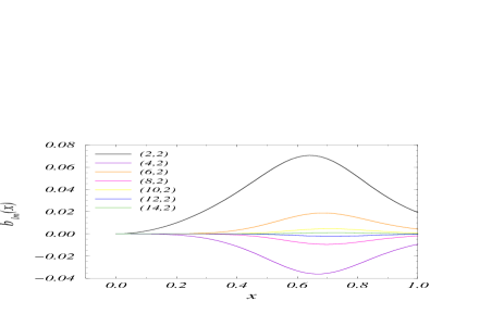
Figure 1: Typical behaviour of the radial part $b_{lm}$ as a function of $l$ for $m=2$. This plot was obtained for $E=-0.18$ and $L=0.44$.

Figure 2: Global phase diagram of the self-gravitating $N$-body system with angular momentum. The dashed lines delimit the region where $\mathcal{H}[S_{N}]$ was computed.

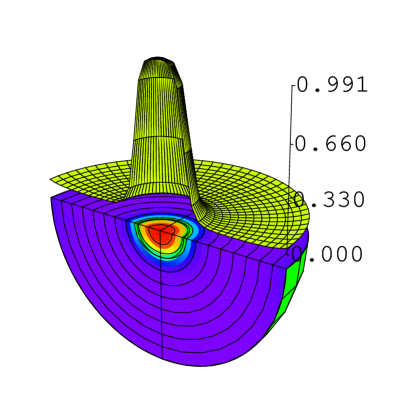
(a) $E=-0.72$, $L=0.4$

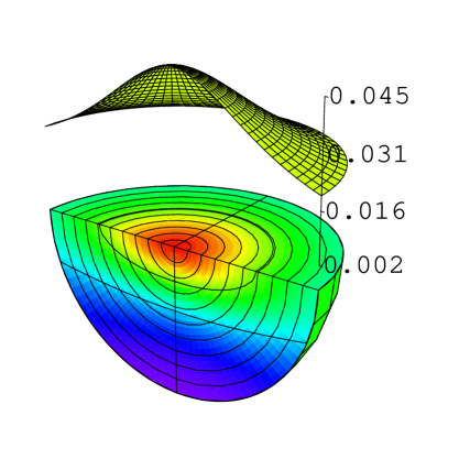
(b) $E=-0.06$, $L=0.4$

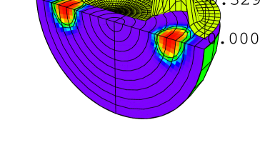
(c) $E=-0.9$, $L=0.5$

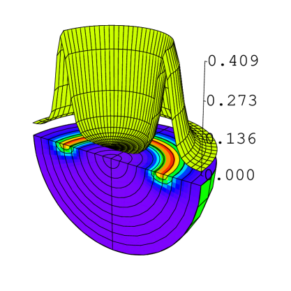
(d) $E=-0.42$, $L=0.5$

Figure 3: Examples of equilibrium distributions $c(\boldsymbol{x})$ occurring inside our spherical box. Shown are the contour plot and, above it, the density profile. The top row corresponds to low angular momentum: one sees single clusters (lower $E$, (a)) and disk-like structures (higher $E$, (b)). The bottom row displays some results for high angular momentum: double clusters (lower $E$, (c)) and rings (higher $E$, (d)). $\boldsymbol{L}$ lies along the vertical axis.

The integral-algebraic system (18) can be solved numerically as follows. Fixing $E$ and $L$ and starting from a reasonable initial guess for $b_{lm}(x)$, one can compute $u_{lm}(x)$ from (17) ($1$-dim. integral). Using this, (18) can be calculated ($2$-dim. integral) to obtain a better form for $b_{lm}(x)$. This scheme can be iterated until convergence. Clearly, numerical calculations must be performed with a finite number of harmonics. A first reduction is obtained by excluding odd harmonics from the calculation. Exclusion of $l=1$ fixes the center of mass in the origin, while absence of higher-order odd harmonics prevents the formation of asymmetric structures (e.g. two clusters of different sizes lying at different distances from the origin). Besides this, from the typical behaviour of $b_{lm}(x)$ obtained from the above procedure, shown in Fig. 1, one clearly sees that $b_{lm}$ dies out fast as $l$ increases. Therefore, all calculations were performed with even harmonics up to and including $l=16$. We set the particles’ masses to one and measured energy and angular momentum in units of $GN^{2}/R$ and $(RGN^{3})^{1/2}$, respectively. Solutions of (13) at fixed $E$ and $L$ were obtained, choosing $\Theta=0.02$ always. For the sake of simplicity, we took the angular momentum parallel to the $3$-axis.

The resulting phase diagram is reported in Fig. 2. In order to discern pure phases from phase-coexistence regions (mixed phases), the Hessian of $S_{N}$, namely

$$\mathcal{H}[S_{N}]=\text{det}\begin{pmatrix}\partial^{2}_{E}S_{N}&\partial_{L}\partial_{E}S_{N}\\ \partial_{E}\partial_{L}S_{N}&\partial_{L}^{2}S_{N}\end{pmatrix}$$ (19)

must be analyzed gross174 ; gross186 . Indeed, in pure phases one has $\mathcal{H}[S_{N}]>0$, while in mixed phases $\mathcal{H}[S_{N}]<0$. In the latter, the specific heat is negative and statistical ensembles (microcanonical and canonical) are inequivalent. For low angular momenta, the system is more likely to be found in a single dense cluster (SC) at low energies, while for higher energies the most probable state is a gaseous cloud (G). The two phases, both pure, are separated by a mixed phase with negative specific heat where different equally-probable equilibrium configurations coexist. One thus recovers the usual collapse scenario thirring70 that is found in theories without angular momentum. For higher angular momenta, instead, the most probable equilibrium configuration is a double cluster (DC, pure phase), although the gas remains the most probable at sufficiently high energies. A sample of equilibrium density profiles is shown in Fig. 3. A central question is clearly that of stability of such structures. A detailed analysis will be given elsewhere, however rings turn out to be unstable, at odds with single and double clusters.

The appearance of the previously-unobserved double-cluster solutions at high angular momenta is particularly remarkable (and stresses again the importance of angular momentum in self-gravitating systems), because in such a state rotational symmetry is spontaneously broken. This is shown explicitly in Fig. 4, where the entropy is plotted as a function of the order parameter $I_{11}-I_{22}$ (measured in units of $NR^{2}$), $I_{ab}$ being the components of the inertia tensor $\mathbb{I}$ ($a,b=1,2,3$). (We remind the reader that we chose the angular momentum to be parallel to the $3$-axis.)

Figure 4: Entropy as a function of the order parameter $I_{11}-I_{22}$ at $L=0.5$ and different values of $E$. The values of $E$ and $L$ correspond to the four markers ($\times$) shown in Fig. 2.

If $L=0$ (or in absence of angular momentum) the system is isotropic ($I_{11}=I_{22}=I_{33}$) and rotational symmetry cannot be broken. When $L\neq 0$, anisotropies may occur ($I_{33}\neq I_{11},I_{22}$) and one can have either rotationally-homogeneous ($I_{11}=I_{22}$) or rotationally-heterogeneous ($I_{11}\neq I_{22}$) solutions. The latter correspond to double clusters. Indeed, the entropy profile develops two peaks at non-zero values of $I_{11}-I_{22}$, corresponding to binary-star systems, with the two stars either aligned on the $1$-axis or on the $2$-axis.

Summarizing, we calculated the static equilibrium density profiles of a self-gravitating and rotating gas using a microcanonical mean-field approach, showing that the formation of double-cluster structures (previously observed only through dynamical approaches) can be obtained from the spontaneous breakdown of a fundamental symmetry of the Hamiltonian (1). We have presented for the first time the global phase diagram as a function of the conserved quantities $E$ and $L$. The inclusion of angular momentum in this analysis is absolutely crucial for these results, the formation of a double-cluster structure being possible only through the spontaneous breaking of a fundamental symmetry of the Hamiltonian (i.e. the rotational symmetry). However, it goes by itself that the formation and stability of stars, double stars, etc. involves other forces (e.g. nuclear and sub-nuclear) than Newtonian gravity, and hence could require other ingredients than just energy and angular momentum contopoulos60 . The results presented here provide nevertheless the most detailed static analysis of the problem to date, and bridge the existing gap between static and dynamical theories. A more exact picture of the situation could be obtained by introducing correlations, which are ignored in the present mean-field approach.

We wish to thank P.-H. Chavanis and O. Fliegans for useful discussions, comments and suggestions.

References

- (1) E-mail: votyakov@hmi.de
- (2) E-mail: demartino@hmi.de
- (3) E-mail: gross@hmi.de
- (4) W. Thirring. Z. Phys. 235 339 (1970)
- (5) D.H.E. Gross. Microcanonical thermodynamics (World Scientific, Singapore, 2001)
- (6) L.D. Landau and E.M. Lifshitz. Statistical physics (Butterworth-Heinemann, Oxford, 1996)
- (7) G. Gallavotti. Statistical mechanics (Springer, Berlin, 1999)
- (8) T. Padmanabhan. Phys. Rep. 188 286 (1990)
- (9) D.H.E. Gross. Phys. Chem. Chem. Phys. 4 863 (2002)
- (10) S. Chandrasekhar. Ellipsoidal figures of equilibrium (Yale University Press, New Haven, 1969)
- (11) D. Lynden-Bell. Mon. Not. R. Astron. Soc. 136 101 (1967)
- (12) P.H. Chavanis, C. Rosier, and C. Sire. Preprint cond–mat/0107345, 2001.
- (13) M. Cerruti-Sola, P. Cipriani, and M. Pettini. Astron. Astrophys. 328 339 (2001)
- (14) P.H. Chavanis. Astron. Astrophys. 381 371 (2002)
- (15) O. Fliegans and D.H.E. Gross. Phys. Rev. E 65 046143 (2002)
- (16) V. Laliena. Phys. Rev. E 59 4786 (1999)
- (17) G. Contopoulos. Z. Astrophys. 49 273 (1960)