Phase transitions in one dimension and less

Abstract

Phase transitions can occur in one-dimensional classical statistical mechanics at non-zero temperature when the number of components $N$ of the spin is infinite. We show how to solve such magnets in one dimension for any $N$, and how the phase transition develops at $N=\infty$. We discuss $SU(N)$ and $Sp(N)$ magnets, where the transition is second-order. In the new high-temperature phase, the correlation length is zero. We also show that for the $SU(N)$ magnet on exactly three sites with periodic boundary conditions, the transition becomes first order.

1 Introduction

It has long been known that phase transitions are uncommon in one-dimensional classical statistical mechanics. An old argument by Peierls shows that in models at non-zero temperature with local interactions and a finite number of degrees of freedom, order is not possible: the entropy gain from disordering the system will always dominate the energy loss. There are (at least) three ways of avoiding this argument. The first two are well understood. A system at zero temperature can of course order: the system just sits in its ground state. A system with long-range interactions can have an energy large enough to dominate the entropy. In this paper, we will discuss in depth a third way of obtaining a phase transition in one dimension. This is to study systems with an infinite number of degrees of freedom per site.

In particular, we will study magnets with $O(N),\ SU(N)$ and $Sp(N)$ symmetry. We will see that there can be a phase transition in the $N\to\infty$ limit. We solve these one-dimensional classical systems for any $N$, and show how the transition occurs only in this limit; for finite $N$ all quantities depend on the temperature analytically. The infinite number of degrees of freedom has roughly the same effect of increasing the effective dimensionality, but the phase transition is very different from those in higher dimension. It is not a phase transition between an ordered phase and a disordered one, but rather between a disordered phase and a seriously-disordered one. In the seriously-disordered phase, the system behaves as if it were at infinite temperature. The entropy has dominated the energy to the point where the energy term does not affect the physics; each spin is effectively independent. The infinite number of degrees of freedom means that this serious disorder is possible even at finite temperature.

The paper is a companion to one by Tchernyshyov and Sondhi [1]. There it is shown that in some magnets, a mean-field calculation yields a phase transition in any dimension. Since mean-field results are exact at $N\to\infty$, this predicts the phase transition we observe here. Their computation also predicts that there is a first-order phase transition for the $SU(N\to\infty)$ magnet on just three sites with periodic boundary conditions. Remarkably, this first-order transition happens only for precisely three sites; for any other number of sites greater than 1 there is a second-order transition.

It has long been known that phase transitions can occur as $N\to\infty$ in zero-dimensional matrix models [2]. Phase transitions in one dimension at infinite $N$ were studied in [3, 4]. In particular, the largest eigenvalue for the $SU(N)$ case discussed here was computed in [4] for any $N$. Here will develop the necessary techniques systematically, and extend these results in several ways. We explicitly find all the eigenvalues of the transfer matrix for these magnets. All these results are completely analytic in $N$ and in the inverse temperature $\beta$ as long as $N$ is finite. The singularity and a phase transition can develop when $N\to\infty$ and $\beta\to\infty$ with $\beta/N$ remaining finite. Knowing all the eigenvalues and their multiplicities explicitly for any $N$ lets us show that there can be a phase transition as $N\to\infty$ even for a finite number of sites in one dimension.

In section 2, we find all the eigenvalues (and their multiplicities) of the transfer matrices in a variety of one-dimensional magnets. In section 3, we use these results to study the phase transitions which occur as the number of sites and $N$ go to infinity. Most of these phase transitions are ferromagnetic, but one is antiferromagnetic. In section 4, we study the first-order transition for the three-site $SU(N)$ chain. In an appendix we collect some useful mathematical results.

2 Solving one-dimensional magnets at any $N$

2.1 The rotor

To illustrate the procedure, we start with a simple rotor, the classical XY model in one dimension. The spin is defined by a periodic variable $0\leq\theta<2\pi$, and spins $\theta$ and $\theta^{\prime}$ on adjacent sites have energy

$$E_{O(2)}(\theta,\theta^{\prime})=-\cos(\theta-\theta^{\prime}).$$ (1)

To compute the partition function of this system, define a transfer “matrix”

$$T(\theta,\theta^{\prime})=e^{-\beta E(\theta,\theta^{\prime})}.$$

Since the variables of the system take continuous values, this isn’t really a matrix, but rather the kernel of an integral operator. It takes functions of $\theta$ to functions of $\theta^{\prime}$ by

$$g(\theta^{\prime})=\int_{0}^{2\pi}\frac{d\theta^{\prime}}{2\pi}\ T(\theta,\theta^{\prime})f(\theta^{\prime}).$$

To compute the partition function, we need eigenvalues $\lambda_{l}$ of $T$. Because the spins take values on a compact space (the circle here), the eigenvalues are discrete and hence labeled by a discrete index $l$. The corresponding eigenfunctions $f_{l}(\theta)$ obey

$$\lambda_{l}f_{l}(\theta^{\prime})=\int_{0}^{2\pi}\frac{d\theta^{\prime}}{2\pi}\ T(\theta,\theta^{\prime})f_{l}(\theta^{\prime}).$$ (2)

For the energy (1), the $f_{l}(\theta)$ are obviously

$$f_{l}=e^{il\theta}.$$

The index $l$ must be an integer to preserve the periodicity under $\theta\to\theta+2\pi$. To see that these are eigenfunctions, note that

$$\lambda e^{il\theta} = \int_{0}^{2\pi}\frac{d\theta^{\prime}}{2\pi}\ e^{\beta\cos(\theta-\theta^{\prime})}e^{il(\theta^{\prime})}$$

$$= \int_{0}^{2\pi}\frac{d\theta^{\prime}}{2\pi}\ e^{\beta\cos(\theta^{\prime})}e^{il(\theta-\theta^{\prime})}.$$

The integral then can be evaluated for any $l$ in terms of a Bessel function:

$$\lambda_{l} = \int_{0}^{2\pi}d\theta^{\prime}\ e^{\beta\cos(\theta^{\prime})}e^{-il\theta^{\prime}}$$ (3)

$$= I_{l}(\beta).$$ (5)

The partition function for $L$ sites with periodic boundary conditions is then

$$Z_{O(2)}=\sum_{l}(I_{l}(\beta))^{L}.$$

When $L$ is large enough, the sum is dominated by largest eigenvalue, which here is the $l=0$ state. The internal energy density $U$ of the system is then

$$U_{O(2)}=-\frac{1}{L}\frac{\partial}{\partial\beta}\ln Z=-\frac{I^{\prime}_{0}(\beta)}{I_{0}(\beta)}.$$

All other quantities such as correlators can easily be found as well, since we have an explicit and complete set of eigenvalues and their multiplicities.

2.2 $O(N)$ magnets

The eigenvalues of the $O(2)$ problem are found by Fourier transforming the transfer matrix. What we need to do for more general cases can be summarized as Fourier analysis on manifolds more general than the circle. In other words, we want to expand a function taking values on a manifold ${\cal M}$ into a series, e.g.

$$T({\cal M})=\sum_{l}\lambda_{l}f_{l}({\cal M})$$

where the $f_{l}({\cal M})$ are complete set of orthonormal functions. The eigenvalues of the transfer matrix are the coefficients of the expansion in this basis.

The problem of Fourier analysis on all the manifolds of interest has been solved already. The key is to exploit the symmetry. A familiar example is where the spins take values on the two-sphere $S^{2}$, where the eigenfunctions are called spherical harmonics. In coset language, the two-sphere can be described as the manifold $S^{2}=O(3)/O(2)$: the $O(3)$ group consists of rotations, while the $O(2)$ subgroup is the set of rotations which leave a given point invariant. Thus different points on $S^{2}$ take values in $O(3)/O(2)$. We parameterize the two-sphere by the usual spherical coordinates: a unit three-vector $\vec{s}\equiv(\sin\theta\sin\phi,\sin\theta\cos\phi,\cos\theta)$. To make progress, it is crucial to consider an energy invariant under the $O(3)$ rotation group, namely

$$E_{O(3)}=-\vec{s}\cdot{\vec{s^{\prime}}}=-\cos\theta\cos\theta^{\prime}-\sin\theta\sin\theta^{\prime}\cos(\phi-\phi^{\prime}).$$

We can expand the transfer matrix energy into irreducible representations of the rotation group, labeled by an angular momentum $l$ and an $L_{z}$ component $m$. The eigenfunctions of the transfer matrix are expressed in terms of Legendre polynomials $P_{l}$, whose explicit definition will be given below. One way of showing that the Legendre polynomials are eigenfunctions of the transfer matrix is to show that they obey an addition theorem, for example

$$P_{l}(\cos\theta\cos\theta^{\prime}+\sin\theta\sin\theta^{\prime}\cos(\phi-\phi^{\prime}))$$

$$\qquad\qquad=P_{l}(\cos\theta)P_{l}(\cos\theta^{\prime})+2\sum_{m=0}^{l}\frac{(l-m)!}{(l+m)!}P_{lm}(\cos\theta)P_{lm}(\cos\theta^{\prime})\cos(\phi-\phi^{\prime}),$$

where the $P_{lm}$ are called associated Legendre polynomials, with $P_{l}=P_{l0}$. One can then expand the function $e^{\beta x}$ in terms of Legendre polynomials, and then use the addition theorem to split the $\theta$ and $\theta^{\prime}$ dependence. This leaves an integral for the eigenvalue.

To just obtain the eigenvalues of the transfer matrix, one does not have to go to all the complications of generalized addition theorems. Mathematicians have developed more in-depth ways of deriving the eigenfunctions, and then the addition theorem comes as a consequence of the computation. A geometric method is discussed in [5], while a much more explicit method is discussed in [6]. We will require the methods of the latter in order to treat the $Sp(N)$ magnet, where the spins do not take values on a symmetric space. (A symmetric space $G/H$ has $H$ a maximal subgroup of $G$; the importance here is that when the spins take values in a symmetric space, the transfer matrix depends on only one parameter.)

First we find the eigenvalues for an $O(N)$-invariant magnet, where the spins $\vec{s}$ take values on the manifold $O(N)/O(N-1)$, which is the $(N-1)$-sphere $S^{N-1}$. We take the energy between nearest neighbors to be

$$E_{O(N)}=-\vec{s}\cdot\vec{s^{\prime}}.$$ (6)

An eigenvalue $\lambda_{l}$ associated with eigenfunction $f_{l}(\vec{s})$ is given by the equation

$$\lambda^{O(N)}_{l}f_{l}(\vec{s})=\int_{S^{N-1}}[D\vec{s^{\prime}}]e^{\beta\vec{s}\cdot\vec{s^{\prime}}}f_{l}(\vec{s^{\prime}}).$$ (7)

where $[D\vec{s^{\prime}}]$ is the usual measure on the $N-1$ sphere, normalized so that $\int[D\vec{s^{\prime}}]=1$. The unit $N$-vector $\vec{s}$ depends on $N-1$ angles, but the energy only depends on the angle between the two spins. This means that to compute the eigenvalue, we need do only one integral. Put in terms of the $O(3)$ spherical harmonics, it means that the eigenvalues depend only the value of $l$ and not $m$. Explicitly, if one sets $\vec{s}=(0,0,\dots,0,1)$, the integrand in (7) depends on only a single angle $\theta$. We can then do the integral over all the other angles in (7), and the measure reduces to [6]

$$\int_{S^{N-1}}[D\vec{s^{\prime}}]=\frac{\Gamma(N/2)}{\Gamma((N-1)/2)\Gamma(1/2)}\int_{0}^{\pi}d\theta\sin^{N-2}\theta$$ (8)

The eigenfunctions for all the magnets we study here can be written in terms of Jacobi polynomials $P^{(\mu,\nu)}_{l}(x)$. These are orthogonal polynomials of order $x^{l}$, and a number of useful properties are collected in the appendix. The eigenfunctions for the $O(N)$ magnet with energy (6) are given by $P^{(r,r)}(\cos\theta),$ where $r=(N-3)/2$. These are often called Gegenbauer or ultraspherical polynomials. They are indeed orthogonal with respect to the measure (8). The eigenvalues are then given by

$$\lambda^{O(N)}_{l}P^{(r,r)}(1)=\frac{\Gamma(N/2)}{\Gamma((N-1)/2)\Gamma(1/2)}\int_{0}^{\pi}d\theta\sin^{N-2}(\theta)e^{\beta\cos\theta}P^{(r,r)}(\cos\theta)$$

Using the integral in the appendix for $\mu=\nu=(N-3)/2$ gives

$$\lambda^{O(N)}_{l}=e^{-\beta}\frac{\Gamma(N/2)\Gamma(N/2-1/2+l)}{\Gamma(1/2)\Gamma(N-1+2l)}M(N/2-1/2+l,N-1+l,2\beta).$$

The function $M$ is called Kummer’s function, and is a confluent hypergeometric function. Its definition and the differential equation it satisfies are given in the appendix. Using the double-argument formula for gamma functions [8] and the identity (37) with $\nu=N/2-1+l$ gives our result

$$\lambda^{O(N)}_{l}=\Gamma(N/2)\left(\frac{\beta}{2}\right)^{N/2-1+l}I_{N/2-1+l}(\beta)$$ (9)

Note that the eigenvalues reduce to the rotor result (5) when $N=2$. Note also that $O(N)$ ferromagnets and antiferromagnets are essentially the same, because redefining $\vec{s}\to-\vec{s}$ for every other spin sends $\beta\to-\beta$. This transformation $\theta\to\pi-\theta$ leaves the measure of the integral invariant, and $\lambda^{O(N)}_{l}(-\beta)=(-1)^{l}\lambda^{O(N)}_{l}(\beta)$.

As a function of $\beta$, the Bessel function is analytic for all $\beta$. Moreover $I_{\gamma}(\beta)>I_{\gamma+1}(\beta)$ for any $\beta$ as long as $\gamma$ is positive. Thus the free energy does not have any singularities as long as $\gamma$ remains finite. One might hope something interesting happens when $N\to\infty$, but in Section 3 we will show that in this case there is still no transition.

2.3 $SU(N)$ magnets

The computation for the $SU(N)$ case is very similar to that of the $O(N)$ case, but we will see in the next section how there is a completely new phase.

The $SU(N)$ magnet is defined in terms of a complex $N$-vector ${z}$ obeying $z^{*}\cdot z=1$. The energy for adjacent sites is

$$E^{SU(N)}=-|z^{*}\cdot z^{\prime}|^{2}.$$ (10)

This energy is not only invariant under global $SU(N)$ rotations, but is invariant under local (gauge) transformations ${z}(x)\to e^{i\alpha(x)}{z}(x)$ at any site $x$. The vector ${z}$ takes values on a complex sphere $U(N)/U(N-1)$, which as a manifold is identical to the real $2N-1$-sphere $O(2N)/O(2N-1)$. However, the $U(1)$ gauge symmetry can be used to effectively reduce the number of degrees of freedom in the problem by 1. For example, one can set the last component of ${z}$ to be real at every site, so ${z}$ effectively takes values on the manifold

$$\frac{U(N)}{U(N-1)\times U(1)}.$$

This manifold is a symmetric space, and is known as the complex projective space $CP^{N-1}$.

Like the $O(N)$ case, the energy between adjacent sites depends only on a single angle $\theta$, where ${z}^{*}\cdot{z^{\prime}}=\cos\theta$ (any phase can always be gauged away). Then the normalized measure can be written as [6, 3]

$$\int_{CP^{N-1}}[D{z^{\prime}}]=2(N-1)\int_{0}^{\pi/2}d\theta\sin^{2N-3}\theta\cos\theta$$ (11)

The eigenvectors of the $CP^{N-1}$ transfer matrix are Jacobi polynomials as well, namely [6, 5]

$$P^{(N-2,0)}_{l}(\cos 2\theta).$$

The $N=2$ case reduces to the ordinary real two-sphere, and indeed the $P^{(0,0)}_{l}$ are ordinary spherical harmonics. The $SU(N)$ symmetry means that the eigenvalues have degeneracies. For example, we saw in section 2.1 that for $N=2$ the eigenvalue depends only on $l$ and not the $S_{z}$ value $m$. For $N=2$, the degeneracy $D_{l}$ of $\lambda_{l}$ is of course $2l+1$; the generalization to all $N$ is [6]

$$D_{l}=\frac{(2l+N-1)\Gamma^{2}(l+N-1)}{\Gamma(N)\Gamma(N-1)\Gamma^{2}(l+1)}$$ (12)

The eigenvalues are given by

$$\lambda^{SU(N)}_{l}P^{(N-2,0)}_{l}(1) = 2(N-1)\int_{0}^{\pi/2}d\theta\sin^{2N-3}\theta\cos\theta\,e^{\beta\cos^{2}\theta}P^{(N-2,0)}_{l}(\cos 2\theta)$$ (13)

$$= \frac{N-1}{2^{N-1}}\int_{-1}^{1}dx(1-x)^{N-2}e^{\beta(1+x)/2}P^{(N-2,0)}_{l}(x)$$ (15)

where $x=\cos 2\theta$. Using the integral in the appendix for $\mu=N-2$, $\nu=0$ gives

$$\lambda^{SU(N)}_{l}=\beta^{l}\frac{\Gamma(N)\Gamma(l+1)}{\Gamma(N+2l)}M(l+1,N+2l,\beta)$$ (16)

For finite $N$ and $\beta$, these are analytic functions. Note that, unlike for $O(N)$ magnets, $\beta>0$ and $\beta<0$ are not equivalent here. For positive $\beta$, we have a ferromagnet: the energy favors aligned spins: a neighbor of $z=(0,0,\ldots,0,1)$ is in the same state $z^{\prime}=z$ (up to a phase). However, $\beta<0$ does not correspond to an antiferromagnet: the energy favors the neighbor $z^{\prime}$ being in any state orthogonal to $z$, i.e., $z^{*}\cdot z^{\prime}=0$. There is a unique orthogonal state only for $N=2$. Thus, with the exception of $SU(2)$, the $SU(N)$ model (10) is ferromagnetic when $\beta>0$, but is not an antiferromagnet when $\beta<0$. For a proper generalization of an antiferromaget, one needs to designate among the $N-1$ vectors orthogonal to $z=(0,0,\ldots,0,1)$ one that can be called “antiparallel” to it, for example, $z^{\prime}=(0,0,\ldots,1,0)$. Doing so manifestly breaks the $SU(N)$ symmetry, as we discuss next.

2.4 $Sp(N)$ magnets

The $SU(2N)$ magnet can be deformed in an interesting way by breaking the $SU(2N)$ symmetry to $Sp(N)$. The main novelty of this $Sp(N)$ magnet is that the phase transition can occur at an antiferromagnetic value of $\beta$. The energy between adjacent sites is

$$E^{Sp(N)}=-a\,|z^{*}\cdot z^{\prime}|^{2}-b\,|zJz^{\prime}|^{2}.$$ (17)

where $z$ is a $2N$-dimensional complex vector, and $J$ is the $2N\times 2N$ dimensional matrix $i\sigma_{y}\otimes I$, where I is the $N$-dimensional identity matrix, and $\sigma_{x}$ the Pauli matrix. The second term breaks the $SU(2N)$ symmetry, but preserves an $Sp(N)$ subgroup. The case $b=0$ reduces to the $SU(2N)$ ferromagnet discussed above. The case $a=0$, studied by Read and Sachdev [7], is a large-$N$ generalization of an antiferromagnet. Indeed, the energy

$$-|zJz^{\prime}|^{2}=-\left|\sum_{i=1}^{N}z_{2i-1}z^{\prime}_{2i}+z_{2i}z^{\prime}_{2i-1}\right|^{2}$$

is minimized when vectors $z$ and $z^{\prime}$ are locked in adjacent flavors $2i-1$ and $2i$, e.g., $z=(0,0,\ldots,0,1)$ and $z^{\prime}=(0,0,\ldots,1,0)$, analogues of spin-down $(0,1)$ and spin-up $(1,0)$ in $SU(2)$.

Like the $SU(N)$ magnet, the generalized model has a local $U(1)$ symmetry. Just like the complex sphere $U(N)/U(N-1)$ is identical as a manifold to the real sphere $O(2N)/O(2N-1)$, the “quaternionic sphere” $Sp(N)/Sp(N-1)$ is identical as a manifold to the complex sphere $U(2N)/U(2N-1)$ (which in turn is equivalent the real $4N-1$-sphere $O(4N)/O(4N-1)$). When we fix a gauge, then $z$ takes values on the manifold

$$\frac{Sp(N)}{Sp(N-1)\times U(1)}.$$ (18)

It is easiest to study first the special point $a=b$, where the gauge symmetry is enhanced to $SU(2)=Sp(1)$. The $SU(2)$ gauge symmetry (a subgroup of the $Sp(2N)$) mixes the $2i-1$ and $2i$ components of $z$ and also mixes $z$ and $z^{*}$. Precisely, if we arrange these components into the matrix

$$M_{i}=\pmatrix{z_{2i-1}&-z^{*}_{2i}\cr z_{2i}&z^{*}_{2i-1}}$$

then all the $M_{i}$ transform under the gauge symmetry as

$$M_{i}\to M_{i}U_{i},$$

where $U_{i}$ is an element of $SU(2)$. The energy is invariant under these transformations even though $U_{i}$ can be different at every point. If we use this symmetry to fix a gauge (e.g. $z_{N-1}=\sin(\theta_{N-1})$, $z_{N}=\cos(\theta_{N-1})$), then $z$ for $a=b$ takes values on the manifold

$$\frac{Sp(N)}{Sp(N-1)\times Sp(1)},$$

which we call $QP^{N-1}$. Solving this case is almost the same as the $SU(N)$ case, because this is a symmetric space. The energy between adjacent sites depends on only one variable, and the measure becomes [6, 3]

$$\int_{QP^{N-1}}[D{z^{\prime}}]=4(N-1)(2N-1)\int_{0}^{\pi/2}d\theta\sin^{4N-5}\theta\cos^{3}\theta$$ (19)

The eigenfunctions of the transfer matrix are the Jacobi polynomials $P^{(2N-3,1)}(\cos 2\theta)$ [6, 5]. Using the integral in the appendix yields

$$\lambda^{QP}_{l}=\beta^{l}\frac{\Gamma(2N)\Gamma(l+2)}{\Gamma(2N+2l)}M(l+2,2N+2l,\beta)$$ (20)

For $N=2$, this is equivalent to the $O(5)$ magnet.

The calculation for $a\neq b$ is more complicated. The reason is that the energy between adjacent sites depends now on two angles: the manifold (18) is not a symmetric space. Luckily, the work of [6] allows us to solve this case as well. It is convenient to write coordinates for the quaternionic sphere $Sp(N)/Sp(N-1)$ in terms of angles $\theta_{i}$ describing an ordinary $N-1$-dimensional sphere, namely

$$q_{1} = \sin\theta_{N-1}\dots\sin\theta_{2}\sin\theta_{1}$$

$$q_{2} = \sin\theta_{N-1}\dots\sin\theta_{2}\cos\theta_{1}$$

$$q_{3} = \sin\theta_{N-1}\dots\sin\theta_{3}\cos\theta_{2}$$

$$\dots$$

$$q_{N-1} = \sin\theta_{N-1}\cos\theta_{N-2}$$

$$q_{N} = \cos\theta_{N-1}$$

Then we have

$$z_{2i-1} = q_{i}e^{i\varphi_{2i-1}}\cos\omega_{i}$$

$$z_{2i} = q_{i}e^{i\varphi_{2i}}\sin\omega_{i}$$

The angles take values in

$$0\leq\theta_{i}\leq\pi/2\qquad\quad 0\leq\omega_{i}\leq\pi/2\qquad\quad 0\leq\varphi_{i}\leq 2\pi.$$

Setting $z_{i}=(0,0,\dots,0,1)$ corresponds to all coordinates $\theta_{i}=\varphi_{i}=\omega_{i}=0$ except $\omega_{N}=\pi/2$. Then the energy (17) is

$$-(a\sin^{2}\omega^{\prime}_{N}+b\cos^{2}\omega^{\prime}_{N})\cos^{2}\theta^{\prime}_{N-1}$$

This indeed depends on two angles, except in the $SU(2)$ gauge-invariant case $a=b$. In terms of these two variables, the measure is

$$\int_{RS}[D{z}]=8(N-1)(2N-1)\int_{0}^{\pi/2}d\theta\sin^{4N-5}\theta\cos^{3}\theta\int_{0}^{\pi/2}d\omega\sin\omega\cos\omega$$ (21)

where we have dropped the now-unnecessary subscripts and primes.

The eigenvectors of the corresponding transfer matrix are now labelled by two indices, $0\leq l^{\prime}\leq l<\infty$. They are written in terms of Jacobi polynomials as [6]

$$\cos^{l-l^{\prime}}\theta\,P^{(0,0)}_{l-l^{\prime}}(\cos 2\omega)P^{(2N-3,l-l^{\prime}+1)}(\cos 2\theta)$$

One can easily check that they are indeed orthogonal with respect to the measure (21). The eigenvalues $\lambda_{ll^{\prime}}$ of the transfer matrix in the Read-Sachdev case $a=0$, $b=1$ are therefore given by

$$\lambda^{RS}_{ll^{\prime}}P^{(0,0)}_{l-l^{\prime}}(1)P^{(2N-3,l-l^{\prime}+1)}(-1)=8(N-1)(2N-1)\int_{0}^{\pi/2}d\theta\sin^{4N-5}\theta\cos^{3}\theta$$

$$\qquad\qquad\qquad\qquad\times\int_{0}^{\pi/2}d\omega\sin\omega\cos\omega e^{\beta\cos^{2}\omega\cos^{2}\theta}P^{(0,0)}_{l-l^{\prime}}(\cos 2\omega)P^{(2N-3,l-l^{\prime}+1)}(\cos 2\theta)$$

Using the integral in the appendix twice, we find that

$$\lambda^{RS}_{ll^{\prime}}=(-\beta)^{l-l^{\prime}}\Gamma(2N)\sum_{j=0}^{\infty}\beta^{j}A_{j}(l,l^{\prime})$$

where

$$A_{j}(l,l^{\prime})=\frac{\Gamma(l-l^{\prime}+1+j)\Gamma(\frac{3}{2}l-\frac{3}{2}l^{\prime}+2+j)\Gamma(\frac{1}{2}l-\frac{1}{2}l^{\prime}+1+j)}{j!\,\Gamma(2l-2l^{\prime}+2+j)\Gamma(\frac{1}{2}l-\frac{3}{2}l^{\prime}+1+j)\Gamma(2N+\frac{1}{2}l+\frac{1}{2}l^{\prime}+j)}$$

This series be rewritten in terms of a confluent hypergeometric function if desired. For the ground state $l=l^{\prime}=0$, it simplifies to

$$\lambda^{RS}_{00}=M(1,2N,\beta).$$

The lowest eigenvalue is identical to that for the $SU(2N)$ magnet, but the general eigenvalues are not the same.

3 Phase transitions as $N\to\infty$

In this section we study systems with the number of sites $L\to\infty$. This means that the free energy follows from the largest eigenvalue $\lambda_{0}$ of the transfer matrix. We saw in the last section that in all cases, $\lambda_{0}$ is analytic function of the inverse temperature $\beta$ for any finite $N$. Thus the only possibility for a phase transition is if this function develops a singularity as $N\to\infty$.

3.1 No transition in the $O(N)$ magnet

It is useful to study the $O(N)$ magnets first. We need to use the asymptotic formula for Bessel functions, valid when $\gamma$ is large [8]:

$$I_{\gamma}(\gamma y)\sim\frac{1}{\sqrt{2\pi\gamma}}\frac{e^{\gamma(\sqrt{1+y^{2}}-\xi^{-1})}}{(1+y^{2})^{1/4}}$$

where

$$\xi^{-1}\equiv\ln(1+\sqrt{1+y^{2}})-\ln(y)$$

This formula implies that to have a non-trivial large $N$ limit, we need to take the inverse temperature $\beta$ to $\infty$ as well, leaving the model in terms of the new variable $y\equiv 2\beta/(N-2)$. Using this formula and some algebra gives the eigenvalue ratios to be

$$\frac{\lambda^{O(N)}_{l+1}(y)}{\lambda^{O(N)}_{l}(y)}=e^{-\xi^{-1}}$$

When we write quantities as a function of $y$, we mean that the expression is valid up to terms of order $1/N$. The two-point function is

$$\langle\vec{s}_{i}\cdot\vec{s}_{i+R}\rangle\propto\left(\frac{\lambda_{1}}{\lambda_{0}}\right)^{R},$$

so $\xi$ is indeed the correlation length. At zero temperature ($y\to\infty$), $\xi$ diverges, just like the one-dimensional Ising model. This is the usual zero-temperature behavior in one-dimensional classical models. The correlation length does not diverge for any other value of temperature, but note that at infinite temperature, $\xi\to 0$. This is a state where the system is completely disordered: every site is essentially independent of any other site, because all configurations have the same weight in the partition sum. It is also useful to compute the internal energy. This is defined as

$$U=-\frac{\partial}{\partial y}\ln\lambda_{0}.$$

Using the asymptotic formula for the Bessel function gives

$$\frac{U^{O(N)}(y)}{N}=\frac{1-\sqrt{1+y^{2}}}{y}$$

In the $N\to\infty$ limit, the internal energy is proportional to $N$, so it is the energy per component which remains finite.

3.2 Transitions in the $SU(N)$ and $Sp(N)$ magnets

The $SU(N)$ and $Sp(N)$ magnets each have a phase transition when $N\to\infty$. The lowest eigenvalue is given by for example

$$\lambda^{SU(N)}_{0}=M(1,N,\beta).$$

As detailed in the last section, for the Read-Sachdev case $\lambda^{RS}_{00}=\lambda^{SU(2N)}_{0}$. To find the large $N$ behavior, it is useful to examine the differential equation (36) for $M(a,N,Ny)$ directly. Then one can see how one can neglect various terms in the equation in various regimes, and then easily solve the equation. This sort of analysis is called boundary-layer theory, and the techniques are discussed at length in [9]. Rewriting (36) in terms of $y=\beta/N$, one has

$$\frac{y}{N}\frac{d^{2}M}{dy^{2}}+(1-y)\frac{dM}{dy}-aM=0.$$ (22)

In the large $N$ limit, we can neglect the first term as long as $y<1$. This shows that

$$\lim_{N\to\infty}M(a,N,Ny)=\frac{1}{(1-y)^{a}}\qquad\hbox{ for }y<1.$$ (23)

This formula can be verified by using Stirling’s formula in the series expression (35) for $M$. The lowest eigenvalue at large $N$ is therefore

$$\lambda^{SU(N)}_{0}(y)\sim\frac{1}{1-y}\qquad\hbox{ for }y<1.$$ (24)

Two important results are apparent from this formula. First, there is a singularity at $y=1$. Second, $U^{SU(N)}(y)$ for $y<1$ does not grow with $N$, and so the internal energy per component vanishes. A vanishing internal energy is characteristic of infinite temperature. The remarkable characteristic of the $SU(N)$ magnet is that this behavior persists all the way from infinite temperature $y=0$ to a finite temperature $y=1$.

In fact, the correlation length vanishes for all $y<1$. This follows from the ratio of the first two eigenvalues:

$$\frac{\lambda^{SU(N)}_{1}(y)}{\lambda^{SU(N)}_{0}(y)} = (Ny)\frac{1}{N(N+1)}\frac{M(2,N+2,Ny)}{M(1,N,Ny)}$$

$$\sim \frac{y}{N(1-y)}\hbox{ for }y<1.$$

As $N\to\infty$, this vanishes if $y<1$. Most scale-invariant critical points have diverging correlation length. At the phase transition at $y=1$, the correlation length vanishes. We call a phase with vanishing correlation length seriously disordered. This distinguishes it from the $y>1$ phase, which is a conventional disordered phase with a finite, non-zero correlation length. In the seriously-disordered phase, the eigenfunction is $P_{0}=1$. This eigenfunction gives equal probabilities to all configurations. Basically, what has happened is that the energy has been swamped by the entropy. For large $N$, there are so many possible spin configurations that if $y<1$, the energy term is too small to make a difference. This is apparent in the integral (15). The measure favors configurations where the angle $\theta$ between nearest-neighbor spins is near $\pi/2$. The reason is as stated before: for a fixed ${z}$, there is only one value of ${z^{\prime}}$ where ${z}^{*}\cdot{z^{\prime}}=1$ but there are many with ${z}^{*}\cdot{z^{\prime}}=0$. The energy favors aligned spins, and at $y=1$ the energy term is strong enough to cause a transition to a phase with finite correlation length. The phase for $y>1$ is still a disordered phase, but a conventional one, as occurs in the $O(N)$ magnets. Note that this phase transition occurs in the ferromagnetic phase ($\beta>0$). If $\beta<0$, the energy and the entropy both favor disorder, so the system is always seriously disordered.

We have asserted but not yet proven that for $y>1$, the internal energy is non-zero and the correlation length is finite. The expression (23) for $M$ in the large-$N$ limit is not valid for $y>1$, because the first term in the differential equation (22) can no longer be neglected when $(y-1)$ is of order $1/\sqrt{N}$. To understand $y>1$, it is useful to derive a differential equation for

$$U=-\frac{\frac{d}{dy}M(1,N,Ny)}{M(1,N,y)}$$

directly. One has

$$y\frac{d}{dy}U = -y\frac{M^{\prime\prime}}{M}+y\left(\frac{M^{\prime}}{M}\right)^{2}$$ (25)

$$= UN(y-1)-N+yU^{2}$$ (27)

where we utilized (22). The internal energy for $y<1$ is a solution of this equation with $U$ finite, found by neglecting the left-hand side and the last term on the right-hand side. It is

$$U^{SU(N)}(y)=\frac{1}{y-1}\qquad\qquad y<1$$

The solution of the differential equation (27) for $N$ large and $y>1$ comes by assuming $U/N$ is finite. Then one neglects the left-hand-side and the second term on the right-hand side, yielding

$$\frac{U^{SU(N)}(y)}{N}=\frac{1-y}{y}\qquad\qquad y>1$$

One can find the $1/N$ corrections to these expressions systematically. For example, one can show that the lowest eigenvalue $\lambda_{0}$ for $y>1$ is to next order in $N$:

$$\lambda_{0}^{SU(N)}(y)=A_{N}e^{N(y-1)}y^{1-N}\qquad\qquad y>1$$ (28)

where $A_{N}=\sqrt{2\pi N}$.

The ratio of the first two eigenvalues for $y>1$ follows from a similar computation, yielding

$$\frac{\lambda^{SU(N)}_{1}(y)}{\lambda^{SU(N)}_{0}(y)} = \frac{y}{N+1}\frac{M(2,N+2,Ny)}{M(1,N,Ny)}$$

$$\sim \frac{y-1}{y}\qquad\qquad y>1$$

Thus we see that the correlation length indeed goes to zero as $y\to 1$ from above. This is a second-order phase transition: the energy is continuous but its derivative is discontinuous. For the Read-Sachdev $Sp(N)$ magnets, the formula is similar:

$$\frac{\lambda^{RS}_{1}(y)}{\lambda^{RS}_{0}(y)} \sim \sqrt{\frac{y-1}{y}}\qquad\qquad y>1$$

3.3 Near the phase transition

The expression for the eigenvalues in terms of the Kummer function $M$ is valid for any value of $y$ and $N$, but the expressions derived for the large-$N$ limit break down when $|y-1|$ is of order $(\sqrt{N})$. All the terms in the differential equations (22,27) need to be included in this region.

To understand the transition region, we study the physics in terms of the variable

$$x\equiv\sqrt{N}(y-1).$$

The differential equation for the lowest eigenvalue (22) becomes (in the $SU(N)$ case)

$$\left(1+\frac{x}{\sqrt{N}}\right)\frac{d^{2}\lambda_{0}}{dx^{2}}-x\frac{d\lambda_{0}}{dx}-\lambda_{0}=0.$$ (29)

For $N$ large, we can neglect the term with the $1/\sqrt{N}$ in it. Thus the subsequent analysis will be valid up to terms of order $1/\sqrt{N}$, as opposed to equations in the last section, which have corrections of order $1/N$. Solving this differential equation by plugging in the series

$$\lambda_{0}=\sum_{j=0}^{\infty}m_{j}x^{j},$$

requires that

$$m_{j+2}=\frac{1}{j+2}m_{j}$$

Plugging this in and summing the series, the solution near $y-1$ for large $N$ is therefore

$$\lambda_{0}=m_{0}e^{x^{2}/2}+m_{1}xM(1,3/2,x^{2}/2)$$ (30)

where the $M$ is indeed our friend the Kummer function. Thus we have shown that the eigenvalue $\lambda_{0}=M(1,N,Ny)$ near $y-1$ at large $N$ is related to a Kummer function with different arguments. To fix the values of $m_{0}$ and $m_{1}$, we need to match this onto the value of $\lambda_{0}$ in the high-temperature phase (24) and in the low-temperature phase (28). From [8], we have the asymptotic formula

$$M(1,3/2,z)\approx\frac{1}{2}\sqrt{\frac{\pi}{z}}e^{z}\qquad\qquad z\hbox{ large}$$

Matching while neglecting terms of order $1/\sqrt{N}$ yields $m_{0}=m_{1}\sqrt{\pi/2}$. Matching this with the numerical result for $A_{N}$ given in the last section gives

$$m_{0}=\sqrt{\frac{\pi N}{2}}\qquad\qquad m_{1}=\sqrt{N}$$

The two terms in (30) cancel when $x$ is large and negative, but add when $x$ is large and positive.

With a little work, one can now derive the specific heat

$$C=\frac{dU}{d(1/y)}$$

everywhere, including at $y=1$. We find $C=1$ for $y<1$, $C=0$ for $y<1$, and $C=1-(2/\pi)$ for $y=1$. The traditional critical exponents can be defined when $N=\infty$. For the specific heat, we have $\alpha=0$, while the correlation length goes to zero logarithmically, so $\nu=0$ as well.

4 First-order transition for three sites

In section 2 we found all the eigenvalues and their degeneracies for the $SU(N)$ magnet. This means that we can also study phase transitions where the number of sites $L$ is finite as well as the infinite-$L$ case studied in section 3. The phase transition persists all the way down to two sites. A remarkable result of the mean-field-theory analysis of [1] is that for three sites (and only for three sites), the transition becomes first-order. We verify this result in this section.

The partition function for the $SU(N)$ magnet with periodic boundary conditions for any number of sites $L$ is given by

$$Z=\sum_{l=0}^{\infty}D_{l}(\lambda_{l})^{L}$$

where the eigenvalues $\lambda_{l}$ and their degeneracies $D_{l}$ are given by (16) and (12) respectively. In this section we study only the $SU(N)$ magnet, so we will omit the $SU(N)$ superscripts. If one takes $L\to\infty$ before taking $N\to\infty$, the partition function is dominated by the largest eigenvalue $\lambda_{0}$ no matter what the degeneracy $D_{l}$ is. However, for finite $L$, the fact that $D_{l}$ grows quite quickly with $l$ and $N$ means that the largest eigenvalue does not necessarily dominate the partition function, but instead

$$Z\approx D_{l_{0}}\lambda_{l_{0}}^{L}$$

for some $l_{0}$ which may not be zero.

All the eigenvalues with finite $l$ (so that $l/N\to 0$ as $N\to\infty$) have the same kind of singularity as $y\to 1$. Thus if the effect of including the degeneracy merely shifts $l_{0}$ to some finite value, the second-order transition remains. To find a first-order transition, we need to study the eigenvalues when $N\to\infty$ with $l/N$ remaining finite. It is convenient to fix the inverse temperature $y$ and study the problem as a function of $r$, defined as

$$r=2\frac{l}{N}.$$

At some value $r=r_{0}$, $D(r)\lambda(r,y)^{L}$ is a maximum; at this value the free energy is minimized (the path integral has a saddle point). The behavior of the eigenvalues at non-zero $r$ can be found by doing a saddle-point approximation to the integral representation of the Kummer function, or by deriving a differential equation for $M^{\prime}/M$ in the manner of (27). To leading order in $N$,

$$\frac{2}{N}\ln(\lambda(r,y)) = A+y-1+\ln(2)+r\ln(y)+(r+1)\ln(r)$$ (33)

$$\qquad-\ln(y-1+A)-(r+1)\ln\left((r+1)^{2}-y+(r+1)A\right)$$

where

$$A=\sqrt{(r+1)^{2}+(y-1)^{2}-1}.$$

At large $N$ and $l$, the degeneracy behaves as

$$\frac{1}{N}\ln(D(r))=(r+2)\ln(r+2)-r\ln(r)-2\ln(2)$$ (34)

The degeneracy is a group-theoretical factor and is independent of the inverse temperature $y$.

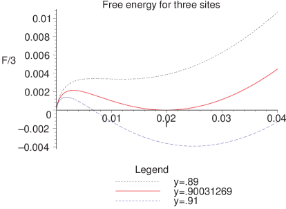
Figure 1: Plots of the free energy per site at and near the first-order transition for three sites

A first-order transition occurs if $r_{0}$ jumps discontinuously as $y$ is varied. What can happen is that $D(r)\lambda(r,y)^{L}$ can develop another maximum as a function of $r$. At some value $y=y_{0}$, one can have two peaks at the same place:

$$D(r_{1})\lambda(r_{1},y_{0})^{L} = D(r_{2})\lambda(r_{2},y_{0})^{L}$$

$$\frac{d}{dr}\left[D(r)\lambda(r,y_{0})^{L}\right]_{r=r_{1}} = \frac{d}{dr}\left[D(r)\lambda(r,y_{0})^{L}\right]_{r=r_{2}}=0.$$

If this happens, the free energy has two minima as a function of $r$. This is the mark of a first-order transition: the internal energy will not be continuous in $y$ because the value of $r_{0}$ jumps from $r_{1}$ to $r_{2}$ as $y$ is varied. We find that for $L=3$, this indeed happens. In Fig. 1, we plot the free energy per site $F/3=-\ln{[D(r)\lambda(r,y)^{3}]}/(3y)$ for values of $y$ just below, above, and at the transitional value $y_{0}=.900312694913\dots$. At the phase transition, the value of $r_{0}$ jumps from $0$ to $.0197950036795\dots$. This is small, but the transition is definitely first order, as shown in [1]. The transition occurs for $y<1$, so the internal energy jumps from $0$ to a finite value. No transition occurs at $y=1$, because the saddle point is already away from $r=0$.

For any other value of $L$, the transition is second-order as before; no second minimum seems to occur. Due to the unwieldiness of the expression (33), we have not been able to prove this in general, but it is easy to see by looking at the curves numerically. Since the first-order transition is so weak for three sites, it would indeed be surprising if the effect of the degeneracies were to overcome the behavior of the eigenvalues for larger $L$. To see this in more detail, let us examine some limits. At large $r$, the eigenvalue goes to zero as $(yr)^{-Nr}e^{Nr}$, while the degeneracy only grows as $r^{2N}$. Thus $r_{0}$ must be finite. The behavior for small $r$ crucially depends on whether $y$ is greater or less than $1$. For $y<1$, $D(0)\lambda(y,0)^{L}=1$, and the slope at $r=0$ is negative. For $y>1$, $D(0)\lambda(y,0)^{L}$ depends on $y$ and the slope at $r=0$ is positive. The simplest behavior for $y<1$ consistent with these limits is to have $D(r)\lambda(y,r)^{L}$ fall off monotonically from $1$ to zero. The simplest behavior for $y>1$ is for $D(r)\lambda(y,r)^{L}$ to rise up to a single maximum at some value $r=r_{0}$, and then fall off to zero for large $r$. By studying plots of the free energy, it seems that this simple scenario is realized for all $L$ larger than $3$. For $L>3$ and $y<1$, $r_{0}=0$, so the partition function is dominated by an eigenvalue with finite $l$. As $y$ is increased past $1$, $r_{0}$ becomes non-zero. There is only a single peak, so $r_{0}$ varies continuously with $y$, so the minimum value of the free energy is also varies continuously. This means that for $L>3$ the only phase transition is a second-order one at $y=1$.

We are very grateful to Shivaji Sondhi for many interesting conversations and for collaboration on [1]. We are also grateful to R. Moessner and N. Read for helpful conversations. The work of P.F. is supported by NSF Grant DMR-0104799, a DOE OJI Award, and a Sloan Foundation Fellowship. O.T. is supported by NSF Grant DMR-9978074.

Appendix A Jacobi polynomials and confluent hypergeometric functions

The Jacobi polynomials $P^{(\mu,\nu)}(x)$ can be expressed in terms of a Rodrigues formula

$$(1-x)^{\mu}(1+x)^{\nu}P^{(\mu,\nu)}_{l}(x)=\frac{(-1)^{l}}{2^{l}l!}\left(\frac{d}{dx}\right)^{l}\left[(1-x)^{l+\mu}(1+x)^{l+\nu}\right]$$

They are defined to be orthogonal with respect to the measure $dx(1-x)^{\mu}(1+x)^{\nu}$:

$$\int_{-1}^{1}dx\,(1-x)^{\mu}(1+x)^{\nu}P^{(\mu,\nu)}_{l}(x)P^{(\mu,\nu)}_{k}(x)=0\qquad\qquad l\neq k$$

Many results on Jacobi polynomials can be found in [10]. One integral we need is [11]

$$\int_{-1}^{1}dx\,(1-x)^{\mu}(1+x)^{\sigma}P^{(\mu,\nu)}_{l}(x)=\frac{2^{\mu+\sigma+1}\Gamma(\sigma+1)\Gamma(\mu+l+1)\Gamma(\sigma-\nu+1)}{l!\ \Gamma(\sigma-\nu-l+1)\Gamma(\mu+\sigma+l+2)}$$

Be aware that there are (different) typos in this formula in both [11] and in [12]. Another useful result is

$$P^{(\mu,\nu)}(1)=\frac{\Gamma(l+\mu+1)}{\Gamma(l+1)\Gamma(\mu+1)}$$

Using these two relations we evaluate the integral

$$\int_{-1}^{1}dx\,(1-x)^{\mu}(1+x)^{\nu}e^{\beta(1+x)}P^{(\mu,\nu)}_{l}(x)$$

$$\qquad\qquad=\sum_{j=0}^{\infty}\frac{\beta^{j}}{j!}\int_{-1}^{1}dx\,(1-x)^{\mu}(1+x)^{\nu+j}P^{(\mu,\nu)}_{l}(x)$$

$$\qquad\qquad=\sum_{j=0}^{\infty}\beta^{j}2^{\mu+\nu+j+1}\frac{\Gamma(\nu+j+1)\Gamma(\mu+l+1)}{l!\,\Gamma(j-l+1)\Gamma(\mu+\nu+j+l+2)}$$

$$\qquad\qquad=P^{(\mu,\nu)}_{l}(1)\,\Gamma(\mu+1)\,\beta^{l}\,\sum_{k=0}^{\infty}(2\beta)^{k}2^{\mu+\nu+l+1}\frac{\Gamma(\nu+k+l+1)}{k!\,\Gamma(\mu+\nu+k+2l+2)}$$

$$\qquad\qquad=P^{(\mu,\nu)}_{l}(1)\,\beta^{l}\,2^{\mu+\nu+l+1}\frac{\Gamma(\mu+1)\Gamma(\nu+l+1)}{\Gamma(\mu+\nu+2l+2)}M(\nu+l+1,\mu+\nu+2l+2,2\beta)$$

where $k=j-l$ and we use the fact that $1/\Gamma(j-l+1)=0$ for $j-l$ a negative integer. The function $M(a,b,z)$ is known as Kummer’s series:

$$M(a,b,z)=\frac{\Gamma(b)}{\Gamma(a)}\sum_{k=0}^{\infty}\frac{z^{k}}{k!}\frac{\Gamma(a+k)}{\Gamma(b+k)}.$$ (35)

The Kummer function is a confluent hypergeometric function because it can be obtained by taking a limit of the hypergeometric function ${}_{2}F_{1}$ where two singularities coincide. It satisfies the differential equation

$$z\frac{d^{2}M}{dz^{2}}+(b-z)\frac{dM}{dz}-aM=0$$ (36)

$M$ is an analytic function of $a,b$ and $z$; the only way to get singularities is to take some or all of these parameters to infinity. A fact useful for $O(N)$ magnets is that the Bessel function $I_{\gamma}(z)$ can be written as

$$I_{\gamma}(z)=\frac{z^{\nu}}{2^{\nu}\,\Gamma(\gamma+1)}e^{-z}M(\gamma+1/2,2\gamma+1,2z)$$ (37)

References

• [1] O.Β Tchernyshyov and S.Β L.Β Sondhi, β€œLiquid-gas and other unusual thermal phase transitions in some large-N magnets” [arXiv:cond-mat/0202128]
• [2] D.Β J.Β Gross and E.Β Witten, Phys.Β Rev.Β D 21 (1980) 446.
• [3] S.Β Hikami and T.Β Maskawa, Prog.Β Theor.Β Phys.Β  67 (1982) 1038.
• [4] A.Β D.Β Sokal and A.Β O.Β Starinets, Nucl.Β Phys.Β B 601 (2001) 425 [arXiv:hep-lat/0011043].
• [5] S.Β Helgason, Groups and Geometric Analysis (Academic, 1984).
• [6] N.Β Vilenkin and A.Β U.Β Klimyk, Representation of Lie groups and special functions, volume 2 (Kluwer, 1991).
• [7] N.Β Read and S.Β Sachdev, Phys.Β Rev.Β Lett.Β 66 (1991) 1773 S.Β Sachdev and N.Β Read, Int.Β J.Β Mod.Β Phys.Β B 5 (1991) 219; S.Β Sachdev, Phys.Β Rev.Β B 45 (1992) 12377.
• [8] Handbook of mathematical functions, with formulas, graphs, and mathematical tables, edited by M.Β Abramowitz and I.Β A.Β Stegun (Dover, 1965).
• [9] C.M.Β Bender and S.A.Β Orszag, Advanced Mathematical Methods for Scientists and Engineers (McGraw-Hill, 1978)
• [10] G.Β SzegΓΆ, Orthogonal Polynomials (AMS, 1975)
• [11] Bateman Manuscript Project, Tables of Integral Transforms (McGraw-Hill, 1954).
• [12] I.S. Gradshtein and I.M. Ryzhik, Table of integrals, series, and products (Academic, 1980).