Ferromagnetism in the Kondo-lattice model

Abstract

We propose a modified RKKY (Rudermann, Kittel, Kasuya, Yosida) technique to evaluate the magnetic properties of the ferromagnetic Kondo-lattice model. Together with a previously developed self-energy approach to the conduction-electron part of the model, we obtain a closed system of equations which can be solved self-consistently. The results allow us to study the conditions for ferromagnetism with respect to the band occupation $n$, the interband exchange coupling $J$ and the temperature $T$. Ferromagnetism appears for relatively low electron (hole) densities, while it is excluded around half-filling ($n=1$). For small $J$ the conventional RKKY theory ($\sim J^{2}$) is reproduced, but with strong deviations for very moderate exchange couplings. For not-too-small $n$ a critical $J_{c}$ is needed to produce ferromagnetism with a finite Curie temperature $T_{\textrm{C}}$, which increases with $J$, then running into a kind of saturation, in order to fall off again and disappear above an upper critical exchange $J$. Spin waves show a uniform softening with rising temperature, and a nonuniform behaviour as functions of $n$ and $J$. The disappearance of ferromagnetism when varying $T$, $J$ and $n$ is uniquely connected to the stiffness constant $D$ becoming negative.

I Introduction

The Kondo-lattice model (KLM)ZEN51 ; AHA55 ; KAS56 ; KON64 ; NAG74 ; NOL79 ; OVC91 ; DDN98 describes the interplay of itinerant electrons in a partially filled conduction band with quantum-mechanical spins (magnetic moments) localized at certain lattice sites. Typical model properties result from an interband exchange between the two subsystems. They are provided by a model Hamiltonian, which consists of two parts:

$$H=H_{s}+H_{sf}.$$ (1)

$H_{s}$ describes uncorrelated electrons in a nondegenerate energy band (”$s$ electrons”)

$$H_{s}=\sum_{ij\sigma}T_{ij}c^{\dagger}_{i\sigma}c_{j\sigma},$$ (2)

where $c^{\dagger}_{i\sigma}(c_{i\sigma})$ creates (annihilates) an electron specified by the lower indices. The index $i$ refers to a lattice site $\mathbf{R}_{i}$, and $\sigma=\uparrow,\downarrow$ is the spin projection. $T_{ij}$ are the hopping integrals. The second term in Eq. (1) represents an interband exchange as an intra-atomic interaction between the itinerant electron spin $\boldsymbol{\sigma}_{i}$ and the localized spin $\mathbf{S}_{i}$ (”$f$ electrons”):

$$H_{sf}=-J\sum_{i}\boldsymbol{\sigma}_{i}\cdot\mathbf{S}_{i}.$$ (3)

According to the sign of the exchange coupling $J$, a parallel ($J>0$) or an antiparallel ($J<0$) alignment of itinerant and localized spin is favored with remarkable differences in the physical properties. We restrict our considerations in the following to the $J>0$ case, sometimes referred to as ”ferromagnetic Kondo-lattice model”, and also known as ”$s-f$ ($s-d$) model”. The applications of the KLM are manifold. In the 1970s it was extensively used to describe the electronic and magneto-optic properties of magnetic semiconductors such as the ferromagnetic EuO and EuS NOL79 ; OVC91 . Most studies focussed on the spectacular temperature dependence of the unoccupied band states. The well-known ”red shift” of the optical absorption edge upon cooling from $T=T_{\textrm{C}}$ to $T=0$ KBJW64 can be understood as a corresponding temperature shift of the lower $5d$ conduction-band edge. Recent quasiparticle band-structure calculation for bulk EuOSNO01a confirm the observed striking temperature dependence as a consequence of a ferromagnetic exchange $J$ of the order of some tenth an eV. The interest in EuO, in particular in thin films, was strongly revived by the observation of a temperature driven metal-insulator transition below $T_{\textrm{C}}$ with a large drop of the resistivity by as much as eight orders of magnitudeSTE01 . This gives rise to a colossal magnetoresistance (CMR) much stronger than that of the manganites as La_1-xSr_xMnO₃. Recently, a surface half-metal-insulator transition was predictedSNO01b for a Eu(100) film. The reason for this is an exchange-split surface state.

In ferromagnetic local moment metals like Gd a RKKY-type interaction is believed to cause the ferromagnetic order, so that in principle a self-consistent description of magnetic and electronic properties by the KLM is possible. The $T=0$-moment of Gd is found to be $7.63\>\mu_{\textrm{B}}$RCM75 . $7\>\mu_{\textrm{B}}$ stems from the exactly half-filled $4f$ shell. The excess moment of $0.63\>\mu_{\textrm{B}}$ is due to an induced spin polarization of the ”a priori” nonmagnetic ($5d,6s$) conduction-bands, indicating a weak or intermediate $J>0$REN99 .

An interesting application of the KLM refers to semimagnetic semiconductors, where randomly distributed Mn²⁺ or Fe²⁺ ions provide localized magnetic moments which influence, via the exchange coupling $J$, the band states of systems like Ga_1-xMn_xAsOHN98 . The Mn²⁺ ions provide both localized spins ($S=\frac{5}{2}$, concentration $x$) and free carriers (holes, concentration $x^{\star}<x$). The latter take care for an indirect coupling between the moments leading for small $x$ even to a ferromagnetic order. The highest $T_{\textrm{C}}$ so far reached is $110$ K for $x=0.053$MOS98 where $x^{\star}$ is found to be about $15\%$ of the Mn concentration $x$. The origin of ferromagnetism in Ga_1-xMn_xAs is controversial. The authors of Ref. MOS98, claimed that the measured $T_{\textrm{C}}(x)$ is consistent with a conventional RKKY interaction between the Mn ions. However, they estimated the exchange coupling $J$ to be of several eV, therewith comparable to the Fermi energy. This makes second order perturbation theory with respect to $J$ rather questionable. RKKY should be modified to account for higher-order spin polarization terms. In this papar we are going to present a respective proposal.

Another modern application of the $J>0$ KLM aims at the manganese oxides with perovskite structures T_1-xD_xMnO₃ (T=La, Pr, Nd; D=Sr,Ca, Ba, Pb) which have attracted great scientific interest because of their CMRJTM94 ; RAM97 . Parent compounds like the protagonist La³⁺Mn³⁺O₃ are antiferromagnetic insulators with a localized Mn spin of $S=2$. Replacing a trivalent La³⁺ ion by a divalent earth-alkali ion (Ca²⁺) leads to a homogenuous valence mixture of the manganese ion (Mn${}^{3+}_{1-x}$, Mn${}^{4+}_{x}$). The three $3d-t_{2g}$ electrons of Mn⁴⁺ can be considered as almost localized, forming an $S=\frac{3}{2}$ spin. Furthermore, ($1-x$) electron per Mn site are of $3d-e_{g}$ type, and itinerant. They are exchange coupled to the $S=\frac{3}{2}$ spins, realizing just the situation which is modelled by the KLM. The exchange coupling is ferromagnetic ($J>0$). Since the manganites are bad electrical conductors, it can be assumed that the intraatomic exchange $J>0$ is much larger than the hopping-matrix element $|t|$. With estimated $e_{g}$ bandwidths of $1-2$ eVSPV96 and lower limits for $J$ of $\begin{array}[]{c}>\\[-6.45831pt] \sim\\[-2.15277pt] \end{array}1$ eVSPV96 , the manganites surely belong to the group of strongly coupled materials. Many fascinating features of the CMR materials can be traced back to an intimate correlation between magnetic and electronic components. One of the not yet fully understood features concerns the spin dynamics in the ferromagnetic phase ($x\sim 0.3$ in La_1-x(Ca,Pb)_xMnO₃). It was reportedPAH96 that the spin wave dispersion (SWD) of materials with high $T_{\textrm{C}}$ (e.g.: La_0.7Pb_0.3MnO₃: $T_{\textrm{C}}=355K$) can be reasonably reproduced by a simple Heisenberg model with nearest-neighbour exchange, only. FurukawaFUR96 gave qualitative arguments that this can be understood for strongly exchange coupled materials. However, strong deviations from the typical Heisenberg behavior of the SWD have been found for manganites with lower $T_{\textrm{C}}$’sHDC98 ; FDH98 ; DHF00 . It is a challenging question whether or not the softening of the SWD at the zone boundary can be explained by a better treatment of the KLM, i.e. by an appropriate consideration of the influence of the conduction-electron self-energy on the effective coupling between the localized magnetic momentsWAN98 ; VSN01 . Solovyev and TerakuraSTE99 argue in such a way claiming that the SWD-softening has a purely magnetic background. By contrast, Mancini et al.MPP00 believe that the KLM [Eq. (1)] has to be extended by a direct (superexchange) interaction between the Mn moments to account for antiferromagnetic tendencies, which dominate the magnetic behaviour of the parent material LaMnO₃.

The above-presented, of course incomplete, list documents the rich variety of, at least, qualitative applications for the KLM. However, the model Hamiltonian [Eq. (1)] provokes such a complicated many-body problem that approximations have to be tolerated. Most of the recent theoretical work on the KLM, aiming at the CMR-materials , assumed classical spinsFUR99 ; MLS95 ; HVO00 , mainly in order to apply ”dynamical mean field theory” (DMFT). It is surely not unfair to consider this assumption as rather problematic.

It is the intention of the present paper to use a special RKKY technique for a detailed investigation of the magnetic properties of the KLM with ferromagnetic interband exchange. We exploit the method of Ref. NRM97, to map the interaction operator $H_{sf}$ [Eq. (3)] to the Heisenberg model Hamiltonian. This is done by averaging out the conduction electron degrees of freedom by properly defined ”restricted” Green functions. The resulting effective Heisenberg exchange integrals are functionals of the itinerant-electron self-energy, and therewith strongly temperature and band occupation dependent. These dependencies manifest themselves in fundamental magnetic properties such as phase diagrams, Curie temperature, spin-wave dispersions and so on.

The electronic self-energy is taken from a ”moment conserving decoupling approach” (MCDA) introduced in Ref. NRM97, and successfully applied to several topics in previous papers SNO01a ; SNO01b ; REN99 ; SMN01 . The method carefully interpolates between nontrivial limiting cases.

The final goal of our effort is to obtain quantitative information about magnetism and the temperature-dependent electronic structure of real local-moment systems. For this purpose it is intended in a future work to combine our model study with a ”first principles” band-structure calculation. First attempts in this direction were done for EuOSNO01a and GdREN99 ; however, the magnetic ordering could not yet be derived self-consistently. The paper is organized as follow. In Sec. II we briefly formulate the many-body problem of the KLM. Section III reproduces the most important aspects of the ”modified RKKY-interaction” (M-RKKY), the understanding of which is vital for a correct interpretation of the results, which are discussed in Sec. IV.

II Kondo-lattice model

The model Hamiltonian [Eq. (1)] provokes a nontrivial many-body problem, which can rigorously be solved only for a small number of limiting cases. For practical reasons, it sometimes appears convenient to use the second quantized form of the exchange interaction [Eq. (3)],

$$H_{sf}=-\frac{1}{2}J\sum_{i\sigma}(z_{\sigma}S^{z}_{i}n_{i\sigma}+S^{\sigma}_{i}c^{\dagger}_{i-\sigma}c_{i\sigma}),$$ (4)

with the abbreviations:

$$n_{i\sigma}=c^{\dagger}_{i\sigma}c_{i\sigma},\>z_{\sigma}=\delta_{\sigma\uparrow}-\delta_{\sigma\downarrow},\>S^{\sigma}_{i}=S^{x}_{i}+iz_{\sigma}S^{y}_{i}.$$ (5)

The first term in Eq. (4) describes an Ising-like interaction between the $z$ components of the localized and the itinerant spin. The second term comprises spin-exchange processes between the two subsystems.

To study the conduction-electron properties we use the single-electron Green function,

$$G_{ij\sigma}(E)=\bigl{\langle}\!\bigl{\langle}c_{i\sigma};c^{\dagger}_{j\sigma}\bigr{\rangle}\!\bigr{\rangle}_{E}.$$ (6)

Its equation of motion reads

$$\sum_{m}\left(E\delta_{im}-T_{im}\right)G_{mj\sigma}(E)=\hbar\delta_{ij}-$$

$$\hskip 50.00008pt-\frac{1}{2}J\{z_{\sigma}I_{ii,j\sigma}(E)+F_{ii,j\sigma}(E)\},$$

where the two types of interaction terms in Eq. (4) are causing the ”spinflip function”

$$F_{im,j\sigma}(E)=\bigl{\langle}\!\bigl{\langle}S^{-\sigma}_{i}c_{m-\sigma};c^{\dagger}_{j\sigma}\bigr{\rangle}\!\bigr{\rangle}_{E}$$ (8)

and the ”Ising function”

$$I_{im,j\sigma}(E)=\bigl{\langle}\!\bigl{\langle}S^{z}_{i}c_{m\sigma};c^{\dagger}_{j\sigma}\bigr{\rangle}\!\bigr{\rangle}_{E}.$$ (9)

These two ”higher” Green functions prevent a direct solution of the equation of motion (II). A formal solution of the Fourier-transformed single-electron Green function,

$$G_{\mathbf{k}\sigma}(E)=\frac{1}{N}\sum_{ij}G_{ij\sigma}(E)\>e^{i\mathbf{k}\cdot(\mathbf{R}_{i}-\mathbf{R}_{j})},$$ (10)

defines the complex electron self-energy $\Sigma_{\mathbf{k}\sigma}(E)$:

$$G_{\mathbf{k}\sigma}(E)=\frac{\hbar}{E+\mu+i0^{+}-\varepsilon(\mathbf{k})-\Sigma_{\mathbf{k}\sigma}(E)},$$ (11)

$$\bigl{\langle}\!\bigl{\langle}[c_{\mathbf{k}\sigma},H_{sf}]_{-};c_{\mathbf{k}\sigma}\bigr{\rangle}\!\bigr{\rangle}_{E}=\Sigma_{\mathbf{k}\sigma}(E)\>G_{\mathbf{k}\sigma}(E).$$ (12)

$\varepsilon(\mathbf{k})$ are the Bloch energies:

$$\varepsilon(\mathbf{k})=\frac{1}{N}\sum_{ij}T_{ij}\>e^{i\mathbf{k}\cdot(\mathbf{R}_{i}-\mathbf{R}_{j})}.$$ (13)

By use of the quasiparticle density of states

$$\rho_{\sigma}(E)=-\frac{1}{\hbar\pi N}\sum_{\mathbf{k}}\text{ Im}G_{\mathbf{k}\sigma}(E-\mu),$$ (14)

we can calculate the spin-dependent occupation numbers

$$\langle n_{\sigma}\rangle=\int\limits^{+\infty}_{-\infty}dE\>f_{-}(E)\>\rho_{\sigma}(E),$$ (15)

important to fix the band polarization $m=\langle n_{\uparrow}\rangle-\langle n_{\downarrow}\rangle$. $f_{-}(E)=\left(\exp(\beta(E-\mu)+1\right)^{-1}$ is the Fermi function.

The central quantity is the self-energy, the determination of which solves the problem. However, for finite temperatures and arbitrary band occupations an exact expression is not avaliable. In Ref. NRM97, a ”moment conserving decoupling approach” (MCDA) predicts the following structure of the self-energy.

$$\Sigma_{\mathbf{k}\sigma}(E)=-\frac{1}{2}Jz_{\sigma}\langle S^{z}\rangle+\frac{1}{4}J^{2}\>D_{\mathbf{k}\sigma}(E).$$ (16)

The first term is linear in the coupling $J$, and proportional to the the local-moment magnetization $\langle S^{z}\rangle$. It represents the result of a mean-field approach which is correct in the weak coupling limit. The second term is predominantly determined by spin-exchange processes between band electrons and localized moments. It is a complicated functional of the self-energy itself. Thus Eq. (16) is not an analytical solution at all, but an implicit equation for $\Sigma_{\mathbf{k}\sigma}(E)$. The MCDA, the detail of which are presented in ref. NRM97, , is a nonperturbational decoupling approach to a set of properly defined Green functions that correctly reproduces the non-trivial exact limiting cases of the KLM. A weighty example is the special case of a ”ferromagnetically saturated semiconductor” SMA81 ; CMI01 ; BJW64 . The various ”higher” Green functions have been approximated by linear combination of ”lower” functions, where the rigorous spectral representations of these ”higher” Green functions and their exact special cases ($S=1/2$, ferromagnetic saturation, …) justify the respective ansatz. Free parameters are finally fitted to exactly known spectral moments. In a certain sense, the method can be considered an interpolation scheme between important limiting cases. It was successfully used in the past for several applicationsSNO01a ; SNO01b ; REN99 ; NRM97 ; SMN01 ; NMR96 . We refer the reader for technical details to one of these papers.

The term $D_{\mathbf{k}\sigma}(E)$ in Eq. (16) contains certain expectations values such as

• $\langle n_{i\sigma}\rangle,\ldots$,

• $\langle S^{z}_{i}\rangle,\>\langle S^{\pm}_{i}S^{\mp}_{i}\rangle,\>\langle(S^{z}_{i})^{2}\rangle$,…,

• $\Delta_{\sigma}=\langle S^{z}_{i}n_{i\sigma}\rangle,\>\gamma_{\sigma}=\langle S^{-\sigma}_{i}c^{\dagger}_{i\sigma}c_{i-\sigma}\rangle$,….

By use of the spectral theorem, terms (a) and (c) can exactly be expressed by the Green functions (6), (8) and (9). Besides Eq. (15) it holds

$$\gamma_{\sigma} = -\frac{1}{\hbar\pi}\int\limits^{+\infty}_{-\infty}dE\>f_{-}(E)\text{ Im}F_{ii,i\sigma}(E-\mu),$$ (17)

$$\Delta_{\sigma} = -\frac{1}{\hbar\pi}\int\limits^{+\infty}_{-\infty}dE\>f_{-}(E)\text{ Im}\Gamma_{ii,i\sigma}(E-\mu).$$ (18)

It remains to express the pure ”local-moment” correlations (b) in terms of the electronic self-energy $\Sigma_{\mathbf{k}\sigma}(E)$ to get a closed system of equations that can be solved self-consistently. A finite coupling between the spin operators must be of indirect nature since the model Hamiltonian [Eq. (1)] does not contain any direct exchange. To obtain the pure spin correlations (b), we map the exchange interaction (4) on an effective Heisenberg model with effective exchange integrals $\hat{J}_{ij}$ being functionals of the electronic self-energy. The result is a ”modified” RKKY interaction (M-RKKY) that takes into account the exchange-induced spin polarization of the band electrons. In lowest order it reproduces the conventional RKKY method.

III Effective Exchange Operator

The starting idea is to map the interband ($s-f$) exchange on an effective spin Hamiltonian of the Heisenberg type.

$$H_{f}=-\sum_{ij}\hat{J}_{ij}\>\mathbf{S}_{i}\cdot\mathbf{S}_{j}.$$ (19)

For this purpose we use the $s-f$ interaction in the folowing form:

$$H_{sf}=-J\frac{\hbar}{N}\sum_{i\sigma\sigma^{\prime}}\sum_{\mathbf{k}\mathbf{q}}e^{-i\mathbf{q}\cdot\mathbf{R}_{i}}\left(\mathbf{S}_{i}\cdot\boldsymbol{\hat{\sigma}}\right)_{\sigma\sigma^{\prime}}c^{\dagger}_{\mathbf{k}+\mathbf{q}\sigma}c_{\mathbf{k}\sigma^{\prime}}.$$ (20)

$\boldsymbol{\hat{\sigma}}$ is the band electron spin operator, the components of which are Pauli spin matrices. The above-mentioned mapping occurs by averaging out the band electron degrees of freedom:

$$H_{sf}\longrightarrow\langle H_{sf}\rangle^{(c)}\equiv H_{f}.$$ (21)

Averaging only in the band electron subspace means that $\langle H_{sf}\rangle^{(c)}$ retains operator character in the $f$-spin subspace. According to Eq. (20) we have to calculate

$$\bigl{\langle}c^{\dagger}_{\mathbf{k}+\mathbf{q}\sigma}c_{\mathbf{k}\sigma^{\prime}}\bigr{\rangle}^{(c)}=\frac{1}{\Xi^{\prime}}\textrm{Tr}\left(e^{-\beta H^{\prime}}c^{\dagger}_{\mathbf{k}+\mathbf{q}\sigma}c_{\mathbf{k}\sigma^{\prime}}\right).$$ (22)

$H^{\prime}$ has exactly the same structure as the KLM Hamiltonian $H$ [Eq. (1)], except for the fact that for the averaging procedure the $f$-spin operators are to be considered as c-numbers, therefore not affecting the trace. $\Xi^{\prime}$ is the corresponding grand partition function. The expectation value [Eq. (22)] does not necessarily vanish for $\mathbf{q}\neq 0$ and for $\sigma\neq\sigma^{\prime}$, as it would do when averaging in the full Hilbert space of the KLM. To calculate Eq. (22) we introduce a proper ”restricted” Green function.

$$\hat{G}^{\sigma^{\prime}\sigma}_{\mathbf{k},\mathbf{k}+\mathbf{q}}(E)=\bigl{\langle}\!\bigl{\langle}c_{\mathbf{k}\sigma^{\prime}};c^{\dagger}_{\mathbf{k}+\mathbf{q}\sigma}\bigr{\rangle}\!\bigr{\rangle}^{(c)}_{E},$$ (23)

which has the ”normal” definition of a retarted Green function, only the averages have to be done in the Hilbert space of $H^{\prime}$. The equation of motion is readily derived for both cases, namely, in the case that $c_{\mathbf{k}\sigma^{\prime}}$ is the active operator or $c^{\dagger}_{\mathbf{k}+\mathbf{q}\sigma}$. By use of the ”free” Green function,

$$G^{(0)}_{\mathbf{k}}(E)=\frac{\hbar}{E+\mu-\varepsilon(\mathbf{k})},$$ (24)

we can combine both equations:

$$\hat{G}^{\sigma^{\prime}\sigma}_{\mathbf{k},\mathbf{k}+\mathbf{q}}(E)=\delta_{\sigma\sigma^{\prime}}\delta_{\mathbf{q},\mathbf{0}}\>G^{(0)}_{\mathbf{k}}(E)-$$

$$-\frac{J}{2N}\!\!\sum_{i\mathbf{k}^{\prime}\sigma^{\prime\prime}}\left\{e^{-i(\mathbf{k}-\mathbf{k}^{\prime})\cdot\mathbf{R}_{i}}G^{(0)}_{\mathbf{k}}(E)\left(\mathbf{S}_{i}\cdot\boldsymbol{\hat{\sigma}}\right)_{\sigma^{\prime}\sigma^{\prime\prime}}\hat{G}^{\sigma^{\prime\prime}\sigma}_{\mathbf{k}^{\prime},\mathbf{k}+\mathbf{q}}(E)\right.$$

$$\hskip 40.00006pt\left.+e^{-i(\mathbf{k}^{\prime}-(\mathbf{k}+\mathbf{q}))\cdot\mathbf{R}_{i}}G^{(0)}_{\mathbf{k}+\mathbf{q}}\left(\mathbf{S}_{i}\cdot\boldsymbol{\hat{\sigma}}\right)_{\sigma^{\prime\prime}\sigma}\hat{G}^{\sigma^{\prime}\sigma^{\prime\prime}}_{\mathbf{k},\mathbf{k}^{\prime}}(E)\right\}.$$

This equation is still exact and can be iterated up to any desired accuracy.

In first order, where the restricted Green function on the right-hand side of [Eq. (III)] is replaced by the ”free” Green function Eq. (24), one obtains

$$\left(\hat{G}^{\sigma^{\prime}\sigma}_{\mathbf{k},\mathbf{k}+\mathbf{q}}(E)\right)^{(1)}=\delta_{\sigma\sigma^{\prime}}\delta_{\mathbf{q},\mathbf{0}}-$$

$$\hskip 40.00006pt-\frac{J}{N}\sum_{i}e^{i\mathbf{q}\cdot\mathbf{R}_{i}}G^{(0)}_{\mathbf{k}}(E)\left(\mathbf{S}_{i}\cdot\boldsymbol{\hat{\sigma}}\right)_{\sigma^{\prime}\sigma}G^{(0)}_{\mathbf{k}+\mathbf{q}}.$$

Exploiting the spectral theorem in the restricted Hilbert space, for the expectation value [Eq. (22)] one finds

$$\left(\frac{1}{N}\sum_{\mathbf{k}}\langle c^{\dagger}_{\mathbf{k}+\mathbf{q}\sigma}c_{\mathbf{k}\sigma^{\prime}}\rangle^{(c)}\right)^{(1)}=\delta_{\sigma\sigma^{\prime}}\delta_{\mathbf{q},\mathbf{0}}\frac{1}{N}\sum_{\mathbf{k}}f_{-}(\varepsilon(\mathbf{k}))\\ -\frac{J}{\hbar}\frac{1}{N}\sum_{i}e^{i\mathbf{q}\cdot\mathbf{R}_{i}}\>D^{(1)}_{\mathbf{q}}\cdot\left(\mathbf{S}_{i}\cdot\boldsymbol{\hat{\sigma}}\right)_{\sigma^{\prime}\sigma}.$$ (27)

Here we have defined

$$D^{(1)}_{\mathbf{q}}=-\frac{1}{\pi}\int\limits^{+\infty}_{-\infty}dE\>f_{-}(E)\text{ Im}\frac{1}{N}\sum_{\mathbf{k}}G^{(0)}_{\mathbf{k}}(E-\mu)G^{(0)}_{\mathbf{k}+\mathbf{q}}(E-\mu).$$ (28)

Because of

$$\mathbf{S}_{i}\cdot\boldsymbol{\hat{\sigma}}=\frac{1}{2}\begin{pmatrix}S^{z}_{i}&S^{-}_{i}\\ S^{+}_{i}&-S^{z}_{i}\end{pmatrix}$$ (29)

one realizes that the first term in Eq. (27) does not contribute to Eq. (21), while the second term gives rise to an effective Hamiltonian like Eq. (19) with the following effective exchange integrals:

$$\hat{J}^{(1)}_{ij}=\frac{1}{N}\sum_{\mathbf{q}}\hat{J}^{(1)}(\mathbf{q})\>e^{-i\mathbf{q}\cdot(\mathbf{R}_{i}-\mathbf{R}_{j})},$$ (30)

$$\hat{J}^{(1)}(\mathbf{q}) = -\frac{1}{2}J^{2}\>D^{(1)}_{\mathbf{q}}$$

$$= -\frac{1}{2}J^{2}\hbar^{2}\sum_{\mathbf{k}}\frac{f_{-}(\varepsilon(\mathbf{k}+\mathbf{q}))-f_{-}(\varepsilon(\mathbf{k}))}{\varepsilon(\mathbf{k}+\mathbf{q})-\varepsilon(\mathbf{k})}.$$

This is the classical RKKY exchange, which comes out in first order of our Green function procedure.

It is well-known that Eq. (III) can be equivalently derived by conventional second-order perturbation theory starting from an unpolarized conduction electron gas. In order to incorporate the exchange-induced spin polarization of the conduction electrons to higher order, it almost suggests itself to modify approximation (III) by replacing in the exact expression [Eq. (III)] the restricted Green function by the full, all polarization processes containing single-electron Green function [Eq. (6)]:

$$\hat{G}^{\sigma^{\prime\prime}\sigma}_{\mathbf{k}^{\prime},\mathbf{k}+\mathbf{q}}(E)\longrightarrow \delta_{\sigma^{\prime\prime}\sigma}\delta_{\mathbf{k}^{\prime}\mathbf{k}+\mathbf{q}}G_{\mathbf{k}+\mathbf{q}\sigma}(E),$$ (32)

$$\hat{G}^{\sigma^{\prime}\sigma^{\prime\prime}}_{\mathbf{k},\mathbf{k}^{\prime}}(E)\longrightarrow \delta_{\sigma^{\prime}\sigma^{\prime\prime}}\delta_{\mathbf{k}\mathbf{k}^{\prime}}G_{\mathbf{k}\sigma^{\prime}}(E).$$ (33)

For the required expectation value [Eq. (22)], we obtain an expression similar to Eq. (27), only $D^{(1)}_{\mathbf{q}}$ has to be replaced by

$$D^{\sigma\sigma^{\prime}}_{\mathbf{q}}=-\frac{1}{\pi}\int\limits^{+\infty}_{-\infty}dE\>f_{-}(E)\text{ Im}\frac{1}{N}\sum_{\mathbf{k}}\times$$

$$\hskip 50.00008pt\times\left(G^{(0)}_{\mathbf{k}}(E-\mu)\>G_{\mathbf{k}+\mathbf{q}\sigma}(E-\mu)+\right.$$

$$\hskip 70.0001pt\left.+G^{(0)}_{\mathbf{k}+\mathbf{q}}(E-\mu)\>G_{\mathbf{k}\sigma^{\prime}}(E-\mu)\right).$$

Exploiting the inversion symmetry, one proves

$$D^{\uparrow\downarrow}_{\mathbf{q}}=D^{\downarrow\uparrow}_{\mathbf{q}}=\frac{1}{2}\sum_{\sigma}D^{\sigma\sigma}_{\mathbf{q}}.$$ (35)

This guarantees an isotropic effective exchange operator Eq. (19) with the exchange-integral

$$\hat{J}(\mathbf{q})=-\frac{J^{2}}{4}\int\limits^{+\infty}_{-\infty}dE\>f_{-}(E)\frac{1}{N}\!\sum_{\mathbf{k}\sigma}\bigg{(}-\frac{1}{\pi}\text{ Im}\Big{(}G^{(0)}_{\mathbf{k}}(E-\mu)\times\Big{.}\bigg{.}\\ \bigg{.}\Big{.}\>\times G_{\mathbf{k}+\mathbf{q}\sigma}(E-\mu)\Big{)}\bigg{)}.$$ (36)

Via $G_{\mathbf{k}+\mathbf{q}\sigma}(E-\mu)$ the effective exchange is a functional of the electronic self-energy Eq. (16), and therefore receives a distinct temperature and electron density dependence.

To obtain the magnetic properties of the local-moment system from the effective operator [Eq. (19)], we use the spin Green function

$$P^{(a)}_{ij}(E)=\bigl{\langle}\!\bigl{\langle}S^{+}_{i};e^{aS^{z}_{j}}S^{-}_{j}\bigr{\rangle}\!\bigr{\rangle}_{E}$$ (37)

first proposed by CallenCAL63 . $a$ is a real number, which eventually helps to derive several spin-correlation functions by applying the spectral theorem to $P^{(a)}_{ij}(E)$ and a proper differentiation with respect to $a$. The equation of motion of $P^{(a)}_{ij}(E)$ reads

$$EP^{(a)}_{ij}(E)=2\hbar\delta_{ij}\langle A_{a}\rangle-2\hbar\sum_{m}\hat{J}_{im}\times\\ \times\bigl{\langle}\!\bigl{\langle}\left(S^{+}_{m}S^{z}_{i}-S^{+}_{i}S^{z}_{m}\right);e^{aS^{z}_{j}}S^{-}_{j}\bigr{\rangle}\!\bigr{\rangle}_{E}.$$ (38)

Here we have abbreviated

$$\langle A_{a}\rangle=\left\langle[S^{+}_{i},e^{aS^{z}_{i}}S^{-}_{i}]_{-}\right\rangle.$$ (39)

It is well-known that a simple random-phase-approximation decoupling of the higher Green function on the right-hand side of Eq. (38) yields surprisingly convincing results in the low- and high- temperature region (”Tyablikov-approximation”). Doing so, after a Fourier-transformation we obtain

$$P^{(a)}_{\mathbf{q}}(E)=\frac{2\hbar^{2}\langle A_{a}\rangle}{E-E(\mathbf{q})+i0^{+}}.$$ (40)

In this approximation the magnon energies $E(\mathbf{q})$ are real:

$$E(\mathbf{q})=2\hbar\langle S^{z}\rangle\bigl{(}\hat{J}_{\mathbf{0}}-\hat{J}(\mathbf{q})\bigr{)},$$ (41)

$$\hat{J}_{0}=\hat{J}(\mathbf{q}=\mathbf{0})=\sum_{i}\hat{J}_{ij}.$$ (42)

Following the Callen-methodCAL63 for the local-moment magnetization one obtains

$$\langle S^{z}\rangle=\hbar\frac{(1+S+\varphi)\>\varphi^{2S+1}+(S+\varphi)\>(1+\varphi)^{2S+1}}{(1+\varphi)^{2S+1}-\varphi^{2S+1}}.$$ (43)

$\varphi$ is the average magnon number,

$$\varphi(S)=\frac{1}{N}\sum_{\mathbf{q}}\frac{1}{e^{\beta E(\mathbf{q})}-1},$$ (44)

which determines $\langle S^{z}\rangle$ and many other spin correlations. Some typical examples are

$$\langle S^{-}S^{+}\rangle = 2\hbar\langle S^{z}\rangle\>\varphi(S),$$ (45)

$$\langle(S^{z})^{3}\rangle = \hbar^{3}S(S+1)\varphi(S)+\hbar^{2}\langle S^{z}\rangle\bigl{(}S(S+1)+\bigr{.}$$ (46)

$$\bigl{.}+\varphi(S)\bigr{)}-\hbar\langle(S^{z})^{2}\rangle\bigl{(}1+3\varphi(S)\bigr{)}.$$

Via Eq. (36) all spin correlations [Eqs. (43)-(46)] are fixed by the electron self-energy [Eq. (16)].

The key quantity of ferromagnetism is the Curie temperature $T_{\textrm{C}}$. Performing the limiting process

$$T\longrightarrow T^{(-)}_{\textrm{C}};\langle S^{z}\rangle\longrightarrow 0^{+}$$ (47)

one finds, from Eq. (43),

$$k_{\textrm{B}}T_{\textrm{C}}=\frac{2}{3}\hbar^{2}S(S+1)\left[\frac{1}{N}\sum_{\mathbf{q}}\left(\hat{J}_{\mathbf{0}}-\hat{J}(\mathbf{q})\right)^{-1}_{T_{\textrm{C}}}\right]^{-1}.$$ (48)

The effective exchange integrals are temperature-dependent and have to be used here for $T\rightarrow T_{\textrm{C}}$.

For the results presented in Sec. IV, we have used the self-energy approach of Ref. NRM97, . The same approach has been applied in Refs. SNO01a, ; SNO01b, ; SMN01, ; REN99, ; MSN01, , so that we can refrain here from presenting details of the method. As explained after Eq. (16) the self-energy of Ref. NRM97, depends on three types of expectation values: purely electronic terms, which are accessible with the single-particle Green function [Eq. (6)]; pure local-spin correlation such as Eqs. (43), (45), (46); and mixed itinerant-electron-local-moment correlations, which are expressible by the ”higher” Green functions [Eqs. (8) and (9)]. Eventually, we have a closed system of equations that can be solved self-consistently for the desired electronic and magnetic properties of the KLM. Some typical results are discussed in Sec. IV.

IV Magnetic Properties

We have evaluated our theory for a s.c. lattice (bandwidth: $W=1$ eV) to find out the magnetic properties of the ferromagnetic KLM. The latter are, however, strongly correlated with the electronic properties, so that they can not be understood without referring to the itinerant-electron subsystem.

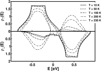
Figure 1: Temperature-dependent quasiparticle density of states $\rho_{\sigma}(E)$ as function of energy (Kondo-lattice model). Parameters: $W=1$ eV, $S=7/2$, $J=0.2$ eV, $n=0.2$. For these parameters the theory yields: $T_{\textrm{C}}=232$ K. The upper half for $\sigma=\uparrow$, the lower half for $\sigma=\downarrow$.

Fig. 1 shows the quasiparticle density of states (QDOS) $\rho_{\sigma}(E)$ for a band occupation $n=0.2$ and a moderate exchange coupling $J=0.2$ eV. The self-consistently determined Curie temperature turns out to be $T_{\textrm{C}}=232K$. In the low-temperature, ferromagnetic phase the QDOS exhibits a remarkable temperature-dependence. For $T\rightarrow 0$ the $\uparrow$ spectrum becomes rather simple (solid line in the upper half of Fig. 1) since the local-moment system is ferromagnetically saturated. A $\uparrow$ electron has therefore no chance to exchange its spin with the localized spins. That means that only the Ising-like interaction term in Eq. (4) really works, leading to a rigid shift of about $-\frac{1}{2}JS$ of $\rho_{\uparrow}(E)$ with respect to the ”free” Bloch DOS $\rho_{0}(E)$. The down-spin QDOS, however, is much more complicated, because a $\downarrow$ electron can exchange its spin with the saturated localized spins. That can, e.g., be done by emitting a magnon $\hbar\omega(\mathbf{q})$, where the electron reverses its spin from $\downarrow$ to $\uparrow$. Consequently, this part of the spectrum (”scattering states”) exactly coincides with $\rho_{\uparrow}(E)$. However, the $\downarrow$ electron has another possibility to exchange its spin with the perfectly aligned localized spins. It can polarize its local spin surrounding by repeated magnon emission and reabsorption. This can even lead to a bound state, which we call the ”magnetic polaron”. For the special case of a single $\downarrow$ electron in an otherwise empty conduction band coupled to a ferromagnetically saturated spin system the formation of the magnetic polaron can rigorously be shown SMA81 ; NDM85 (see Fig. 1 in Ref. MSN01, ). Formation of a polaron costs more energy than magnon emission. Polaron states therefore build the upper part of the $\downarrow$ spectrum.

Magnon emission by the $\downarrow$ electron is equivalent to magnon absorption of a $\uparrow$ electron, with one exception: magnon absorption can occur only if there are magnons in the system. This is not the case at $T=0$ in the ferromagnetic saturation. At finite temperature, however, there are magnons to be absorbed by $\uparrow$ electrons. Consequently, scattering states appear in the $\uparrow$ spectrum too. Because of the possible spin exchange both spin spectra occupy exactly the same energy region at all $T>0$. It is interesting to observe that even for such a moderate coupling $J=0.2$ eV ($W=1$ eV) there opens a gap between a lower and an upper quasiparticle subband. In the lower subband the electron hops mainly over lattice sites, where it orients its spin parallel to the local moment, either without or with preceding spin-flip by magnon emission (absorption). The upper subband consists of polaron states with finite lifetimes. Note that such elementary processes are not recognizable when for mathematical simplicity classical spins ($S\rightarrow\infty$) are assumed FUR99 ; MLS95 ; HVO00 . The QDOS in Fig. 1 clearly demonstrates that the conduction electrons are not at all fully spin polarized as is often used in DMFT treatments of the KLMFUR96 ; HVO00 . That is true only in the unphysical limit $S\rightarrow\infty.$

Let us now concentrate the rest of the discussion on the magnetic properties of the KLM. They are determined by the respective behaviour of the effective exchange integrals $\hat{J}_{ij}$.

Fig. 2 shows the distance dependence of $\hat{J}_{ij}$ as it follows from the conventional RKKY [Eq. (30)]. We recognize the well-known oscillating and long-range behavior. According to Eq. (III) two parameters influence the oscillation: the interband exchange $J$ and the band occupation $n$. The ”amplitude” of the oscillation is proportional to $J^{2}$, while the ”period” is fixed via the chemical potential $\mu$ by the conduction electron density $n$. A remarkable temperature dependence is not observed.

The oscillations of the effective exchange integrals $\hat{J}_{ij}$ are

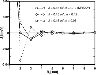
Figure 2: Conventional RKKY exchange integrals $\hat{J}_{ij}$ as a function of the distance $R_{ij}$ between lattice sites in (100) direction for various band occupation $n$ and different interband exchange couplings $J$. Parameters: $T=0K$, $W=1$ eV, s.c. lattice. For comparison a respective example of the modified RKKY model is included.

less regular when higher-order polarization effects in the conduction band are taken into account [Eq. (36)]. Fig. 3 and Fig. 4 show two examples for two different $J$’s and several band occupations $n$.

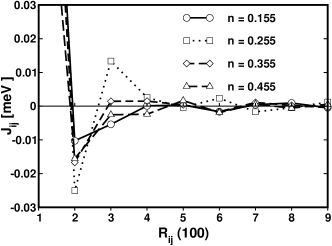
Figure 3: Effective exchange integrals $\hat{J}_{ij}$ of the ”modified” RKKY model as a function of the distance $R_{ij}$ in (100) direction for various band occupations. Parameters: $T=0K$, $J=0.1$ eV, $W=1$ eV, s.c. lattice, $S=7/2$.

The nonregular $J$ dependence results from the fact, that $J$ appears in Eq. (36) not only as a prefactor $J^{2}$ but also in a complicated manner via the Green function $G_{\mathbf{k}+\mathbf{q}\sigma}(E-\mu)$ of the polarized itinerant electron system. Of similar complexity is the $n$ dependence. In the conventional RKKY [Eq. (III)] it comes into play only through the chemical potential in the Fermi function, while in the full expression [Eq. (36)], several correlation functions as $\langle n_{\sigma}\rangle$, $\langle S^{z}n_{\sigma}\rangle$, $\langle S^{-\sigma}c^{\dagger}_{\sigma}c_{-\sigma}\rangle$,…[Eqs. (15), (17), (18)] contribute to the $n$ dependence.

Figure 4: The same as in Fig. 3, but for $J=0.2$ eV.

To demonstrate the influence of the interband exchange coupling $J$ on the effective Heisenberg-exchange integrals $\hat{J}_{ij}$ in more detail, in Fig. 5 we plot the $J$ dependence of $J_{x}$, $x=1,\ldots,9$. $J_{x}$ is the effective exchange integral between sites separated along the (100) direction by $x$ lattice constants..

Figure 5: Effective exchange integrals $J_{x}$ between $x$th nearest neighbors ($x=1,2,\ldots,9$) in (100) direction (s.c. lattice) as a function of the interband exchange coupling $J$. Parameters: $T=0$ K, $n=0.2$, $W=1$ eV, $S=7/2$. Note the different energy scales.

$J_{4},\ldots,J_{9}$ show an oscillatory structure in the weak-coupling region, being, one order of magnitude smaller than $J_{2,3}$ and even two orders of magnitude smaller than $J_{1}$. For $J>0.2$ eV $J_{3},\ldots,J_{9}$ are so strongly damped that the magnetism of the KLM can be described by a Heisenberg model with next- and next-nearest-neighbor exchanges only. In the weak-coupling regime, however, the higher terms $J_{3},\ldots,J_{9}$ can not be neglected. Similar statements can be found inFUR96 . Maybe this is an explanation why CMR materials with high $T_{\textrm{C}}$ can be described reasonably wellPAH96 by a short-range Heisenberg model, while other materials with lower $T_{\textrm{C}}$ exhibit strong deviationsHDC98 ; FDH98 ; DHF00 . In any case the main contribution to the exchange coupling stems from the next-nearest-neighbors. $J_{1}$ determines the stable magnetic configuration. The negative slope of $J_{1}$ for $J>0.5$ eV indicates already a breakdown of the ferromagnetic order, which is more carefully inspected below.

The effective exchange integrals $J_{x}$ exhibit an interesting electron-density dependence (Fig. 6). For low densities up to $n=0.3$ only $J_{1}$ is of importance. A Heisenberg model with nearest-neighbour exchange will appropriately describe the magnetic properties of the KLM.

Figure 6: The same effective exchange integrals as in Fig. 5, but now as a function of the band occupation $n$ for $J=0.2$ eV.

For larger $n$, however, the exchange interaction becomes very long-range, even $J_{9}$ is not negligible. From Fig. 5 and 6 we learn that the interplay between local interband exchange $J$ and band occupation $n$ does lead to a rather complicated behaviour of the effective RKKY exchange integrals.

The effective exchange integrals determine the magnetic properties of the KLM. On the other hand, they depend on the electron self-energy which is strongly influenced by magnetic correlation functions. Typical examples of the latter are plotted in Fig. 7, calculated for $n=0.2$ and $J=0.2$ eV.

Figure 7: Several spin correlation functions of the local-moment system in dependence on the temperature $T$. Parameters: $J=0.2$ eV, $n=0.2$, $S=7/2$, s.c. lattice, $W=1$ eV. The theory, presented in the text, self-consistently yields $T_{\textrm{C}}=232$ K.

The electronic part of the self-consistent solution, represented by the temperature dependent QDOS, is shown in Fig. 1. The Curie temperature is found as $T_{\textrm{C}}=232$ K. The local-moment magnetization $\langle S^{z}\rangle$ is of Brillouin function type, and the qualitative shapes of the other spin correlations are also familiar from the pure Heisenberg model.

The key-quantity of ferromagnetism is the Curie temperature $T_{\textrm{C}}$. $T_{\textrm{C}}>0$ comes out as a consequence of an indirect coupling between the local moments, mediated by spin polarization of itinerant electrons. Therefore, a strong particle density dependence of $T_{\textrm{C}}$ has to be expected. Figure 8 shows $T_{\textrm{C}}(n)$ for various $J$ from the weak to moderate coupling regime, calculated according to [Eq. (48)].

Figure 8: Curie temperature as a function of the band occupation $n$ for various interband exchange couplings ($S=7/2$, s.c. lattice, $W=1$ eV), calculated by use of the ”modified” RKKY. model.

Ferromagnetism appears for low particle (hole) densities, where the ferromagnetic region increases with increasing $J$. The $T_{\textrm{C}}$ values are of realistic order. A similar $n$ dependence of $T_{\textrm{C}}$ has been found in Ref. CMI01, within an extended multi-band KLM. No ferromagnetism appears around half-filling ($n=1$). It can be speculated that antiferromagnetism, which is not considered within our approach, becomes stable near $n=1$. It is

Figure 9: The same as in Fig. 8, but calculated by use of the ”conventional” RKKY model.

interesting to compare the results of Fig. 8 with their conterparts from conventional RKKY (Fig. 9), using the same model parameters and the same $T_{\textrm{C}}$-formula [Eq. (48)]. The $T_{\textrm{C}}$ values are higher, but the region of $n$ where ferromagnetism appears, is distinctly narrower. The critical $n$, where $T_{\textrm{C}}$ vanishes again, is independent of $J$, in contrast to the full theory in Fig. 8.

The Curie temperature shows a remarkable $J$ dependence, which is plotted in Fig. 10 for various band occupations. According to conventional RKKY theory one would expect a monotonic increase of $T_{\textrm{C}}$ with increasing $J$. A mean-field evaluation of the effective Heisenberg model would lead to $T_{\textrm{C}}\sim J^{2}$.

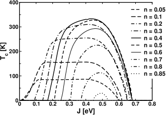
Figure 10: Curie temperature as a function of the interband exchange coupling $J$ for various band occupations $n$ ($S=7/2$, s.c. lattice, $W=1$ eV).

Our theory becomes identical to conventional RKKY theory for small $J$. However, because of the random-phase-approximation (RPA) treatment of the Heisenberg operator [Eq. (19)], there are deviations of $T_{\textrm{C}}$ from the $J^{2}$ behavior even for small $J$. A more important and very characteristic feature of our modified RKKY approach is the appearence of a critical coupling $J_{c}$ for band occupations $n\geq 0.13$, below which no ferromagnetism occurs. This occurs for band fillings, for which conventional RKKY theory fails to yield a ferromagnetic RPA solution (Fig. 9). Therefore the existence of $J_{c}$ does not disprove the agreement of conventional and modified RKKY theory for small $J$. After a steep increase as function of $J$, $T_{\textrm{C}}$ runs into a kind of saturation, where the plateau becomes smaller the larger the bandfilling $n$. With a further increase of $J$, the Curie temperature again decreases and disappears at an upper critical $J$ value. The upper critical value of $J$ coincides with the point where the stiffness constant $D$ of the spin-wave dispersion [Eq. (41)] ($E(\mathbf{q})\approx D\>\mathbf{q}^{2}$ near the $\Gamma$ point) becomes negative due to a respective behavior of the dominating effective exchange integrals $J_{1},J_{2},J_{3}$ (see inset in Fig. 5 and Eq. (48)). It can be suspected that for larger $J$ the local-moment system becomes antiferromagnetic. Furthermore, it cannot be excluded that for still larger $J$’s the system returns to ferromagnetism. These features are far beyond conventional RKKY theory and due to higher order polarization terms, which come into play via the full Green function $G_{\mathbf{k}+\mathbf{q}\sigma}(E-\mu)$ in the expression (36) for the effective exchange integral $\hat{J}(\mathbf{q})$. The manganites are often treated as ferromagnets with $J\rightarrow\infty$ in the KLMFUR96 . According to Fig. 10 this must be reexamined. For $J\approx W$ ferromagnetism is unlikely in the KLM.

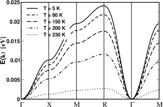
Figure 11: Spin-wave dispersion of the ferromagnetic Kondo-lattice model as a function of the wave vector for different temperatures $T$. Parameters: $J=0.2$ eV, $n=0.2$, $S=7/2$, s.c. lattice, $W=1eV$. The self-consistently calculated Curie temperature is $T_{\textrm{C}}=232$ K.

The spin-wave dispersion, plotted in Fig. 11 for the main symmetry direction, obtains, via the effective exchange integrals a distinct temperature dependence. Upon heating the dispersion relation uniformly softens, disappearing above $T_{\textrm{C}}$. This agrees qualitatively with the a neutron-scattering study of the spin dynamics in the manganite Pr_0.63Sr_0.37MnO₃HDC98 . However, we do not share the view of the authors of Ref. HDC98, , i.e., that the unexcepted results rule out a simple Heisenberg Hamiltonian. In our opinion the Heisenberg model works as long as the exchange integrals are renormalized in a proper way by the conduction-electron self-energy.

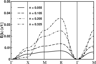
Figure 12: The same as in Fig. 11, but for different band occupations at $T=0$ K.

Changing the doping in the III-V based diluted magnetic semiconductors such as Ga_1-xMn_xAs, or in manganites like La_1-xCa_xMnO₃, does alter the band occupation and therewith the physics of these materials. It is therefore worthwhile to inspect the $n$ dependence of the spin-wave dispersion. This is done in Fig. 12 for low bandoccupations and in Fig. 13 for higher band occupations for a model system with $J=0.2$ eV. For low densities (Fig. 12) we observe a strengthening of the magnon dispersion with increasing band filling, while the opposite is true for stronger fillings (Fig. 13). This is in accordance with the $T_{\textrm{C}}$ behavior of Fig. 8. The band occupation $n=0.485$ is very close to the upper critical point of the $J=0.2$ eV curve in Fig. 8. The corresponding spin-wave dispersion in Fig. 13 shows a strong softening. A slightly higher $n$ leads to parts of the Brillouin zone with negative magnon energies, i.e. the ferromagnetic ground state becomes unstable. The stiffness $D$, defined by $E(\mathbf{q})\approx D\>\mathbf{q}^{2}$ for $\mathbf{q}\rightarrow\mathbf{0}$, becomes negative. The points where $D=D(n,J,T=0)=0^{+}$ exactly coincide in our theory with those for which $T_{\textrm{C}}=T_{\textrm{C}}(n,J)\rightarrow 0$, directly derived from the local-moment magnetization $\langle S^{z}\rangle$. Qualitatively the same $n$ dependence of the spin-wave dispersion is reported in Ref. WMH98, .

Figure 13: The same as in Fig. 12, but for higher band occupations.

An example for the $J$ dependence of the spin-wave dispersion is presented in Fig. 14 ($n=0.2$, $T=0$ K, $S=\frac{7}{2}$). Again we observe a strengthening of the dispersion

Figure 14: The same as in Fig. 11, but for different interband exchange couplings $J$ at $T=0$ K.

with $J$ when $T_{\textrm{C}}$ increases simultaneously, and a softening, when $T_{\textrm{C}}$ decreases (see Fig. 10).

V Summary

We have evaluated an approximate but self-consistent theory for a local-moment ferromagnet described within the framework of the ferromagnetic Kondo-lattice model. Candidates for this model are magnetic semiconductors (EuO, EuS), diluted magnetic semiconductors (Ga_1-xMn_xAs), magnetic metals (Gd, Dy, Tb) and CMR materials (La_1-xCa_xMnO₃). We have used a previously developed Green function techniqueNRM97 for a detailed investigation of the magnetic properties of the exchange-coupled local moment-itinerant electron system. An extended RKKY mechanism has been worked out to derive magnetic phase diagrams as well as spin-wave dispersions. The latter show strong dependencies on temperature (uniform softening for $T\rightarrow T_{\textrm{C}}$), on the band occupation $n$, and on the exchange coupling $J$. These dependencies are due to the respective behaviors of the effective exchange integrals between the localized moments. The effective exchange integrals are found by mapping the interband exchange ($s-f$) coupling, characteristic of the KLM, to an effective Heisenberg model. They turn out to be functions of the electronic self-energy, being therewith strongly temperature and electron density dependent. For small $J$ our theory reproduces the results of the well-known conventional RKKY treatment, which represents second-order perturbation theory to the KLM. Already for very moderate $J$, however, substantial deviations appear, when higher-order terms of the induced conduction-electron spin polarization bring their influence to bear.

For the future the presented approach has to be extended to antiferromagnetic moment configurations in order to complete the phase diagram. Furthermore, Coulomb correlations have to be introduced for the conduction-electron subsystem. Their neglect in the original KLM seems to be only poorly justified.

It is further intended to apply the modified RKKY procedure to the antiferromagnetic KLM ($J<0$) in order to investigate the interplay between ”Kondo screening” and RKKY. This, however, requires a serious check whether or not the MCDA in its present formNRM97 is able to account for the subtle low-temperature (Kondo) physics.

References

- (1) C. Zener, Phys. Rev. 81, 440 (1951).
- (2) P. W. Anderson and H. Hasegawa, Phys. Rev. 100, 675 (1955).
- (3) T. Kasuya, Prog. Theor. Phys. 16, 45 (1956).
- (4) J. Kondo, Prog. Theor. Phys. 32, 37 (1964).
- (5) E. L. Nagaev, phys. stat. sol. (b) 65, 11 (1974).
- (6) W. Nolting, phys. stat. sol. (b) 96, 11 (1979).
- (7) S. G. Ovchinnikov, Phase Transitions 36, 15 (1991).
- (8) M. Donath, P. A. Dowben, and W. Nolting, eds., Magnetism and Electronic Correlations in Local-Moment Systems; Rare-Earth Elements and Compounds (World Scientific, Singapore, 1998).
- (9) G. Busch, P. Junod, and P. Wachter, Phys. Lett. 12, 11 (1964).
- (10) R. Schiller and W. Nolting, Solid State Commun. 118, 173 (2001).
- (11) P. G. Steeneken, L. H. Tjeng, I. Elfimov, G. A. Sawatzky, G. Ghiringhelli, N. B. Brookes, and D.-J. Huan, cond-mat/ 0105527 (2001).
- (12) R. Schiller and W. Nolting, Phys. Rev. Lett. 86, 3847 (2001).
- (13) L. W. Roeland, G. J. Cock, F. A. Muller, C. A. Moleman, K. A. M. McEwen, R. C. Jordan, and D. W. Jones, J. Phys. F 5, L233 (1975).
- (14) S. Rex, V. Eyert, and W. Nolting, J. Magn. Magn. Mat. 192, 529 (1999).
- (15) H. Ohno, Science 281, 951 (1998).
- (16) F. Matsukura, H. Ohno, A. Shen, and Y. Sugawara, Phys. Rev. B 57, R2037 (1998).
- (17) S. Jin, T. H. Tiefel, M. McCorneck, R. A. Fastnacht, R. Ramesh, and L. H. Chen, Science 264, 413 (1994).
- (18) A. P. Ramirez, J. Phys.: Condens. Matter 9, 8171 (1997).
- (19) S. Satpathy, Z. S. Popovic, and F. R. Vukajlovic, Phys. Rev. Lett. 76, 960 (1996).
- (20) T. G. Perring, G. Aeppli, S. M. Hayden, S. A. Carter, J. P. Remeika, and S.-W. Cheong, Phys. Rev. Lett. 77, 711 (1996).
- (21) N. Furukawa, J. Phys. Soc. Japan 65, 1174 (1996).
- (22) H. Y. Hwang, P. Dai, S.-W. Cheong, G. Aeppli, D. A. Tennant, and H. A. Mook, Phys. Rev. Lett. 80, 1316 (1998).
- (23) J. A. Fernandez-Baca, P. Dai, H. Y. Hwang, C. Kloc, and S.-W. Cheong, Phys. Rev. Lett. 80, 4012 (1998).
- (24) P. Dai, H. Y. Hwang, J. Zhang, J. A. Fernandez-Baca, S.-W. Cheong, C. Kloc, Y. Tomioka, and Y. Tokura, Phys. Rev. B 61, 9553 (2000).
- (25) X. Wang, Phys. Rev. B 57, 7427 (1998).
- (26) M. Vogt, C. Santos, and W. Nolting, phys. stat. sol. (b) 223, 679 (2001).
- (27) I. V. Solovyev and K. Terakura, Phys. Rev. Lett. 82, 2959 (1999).
- (28) F. Mancini, N. B. Perkins, and N. M. Plakida, cond-mat/ 0011464 (2000).
- (29) N. Furukawa, Physics of Manganites (Plenum, New York, 1999), p. 1.
- (30) A. J. Millis, P. B. Littlewood, and B. I. Shraiman, Phys. Rev. Lett. 74, 5144 (1995).
- (31) K. Held and D. Vollhardt, Phys. Rev. Lett. 84, 5168 (2000), the authors incorporate a Hubbard-interaction between the conduction electrons;”correlated KLM”.
- (32) D. Meyer, C. Santos, and W. Nolting, J. Phys.: Condens. Matter 13, 2531 (2001).
- (33) W. Nolting, S. Mathi Jaya, and S. Rex, Phys. Rev. B 54, 14455 (1996).
- (34) W. Nolting, S. Rex, and S. M. Jaya, J. Phys.: Condens. Matter 9, 1301 (1997).
- (35) H. B. Callen, Phys. Rev. 130, 890 (1963).
- (36) R. Schiller, W. Müller, and W. Nolting, Phys. Rev. B 64, 134409 (2001).
- (37) B. S. Shastry and D. C. Mattis, Phys. Rev. B 24, 5340 (1981).
- (38) W. Nolting, U. Dubil, and M. Matlak, J. Phys.: Condens. Matter 18, 3687 (1985).
- (39) A. Chattopadhyay and A. J. Millis, Phys. Rev. B 64, 024424 (2001).
- (40) P. Wurth and E. Müller-Hartmann, Europ. Phys. J. B 5, 403 (1998).