Anomalously Soft Droplets and Aging in Short-ranged Spin Glasses

Abstract

We extend the standard droplet scaling theory for isothermal aging in spin glasses assuming that the effective stiffness constant of droplets as large as extended defects is vanishingly small. A novel dynamical order parameter $q_{\rm D}$ and the associated dynamical susceptibility $\chi_{\rm D}$ emerge. Breaking of the fluctuation dissipation theorem takes place at $q_{\rm D}$ well below the equilibrium Edwards-Anderson order parameter $q_{\rm EA}(>q_{\rm D})$ at which the time translational invariance is strongly broken. The scenario is examined numerically in a 4 dimensional EA Ising spin glass model.

Recently aging in spin glasses APY-review ; Saclay ; Uppsala ; Review-Rieger ; BCKM has attracted renewed interest both in experimental, numerical and theoretical studies. The phenomena provide very interesting and almost the only realistic way to explore large scale, non-trivial properties of glassy phases. A major theoretical progress was the development of dynamical mean-field theories (MFT) for spin glasses and related systems MFT which lead to findings of some novel view points in glassy dynamics such as the concept of effective temperature CKP97 . However, the MFT themselves do not provide insights into what will become important in realistic finite dimensional systems, such as nucleation processes.

The droplet theory BM ; FH1 ; FH2 developed a scaling theory assuming droplet excitations as basic nucleation processes. It provides a perspective for equilibrium and dynamical properties of finite dimensional spin glasses. Though it was developed more than a decade ago, many of its predictions have remained to be clarified.

Recently, anomalous low energy and large scale excitations were found LEE in active studies of spin-glass models at $T=0$. In the present letter, we develop a refined scenario for isothermal aging in spin glasses where such anomalous low energy excitations play a significant role. Most importantly, it explains the fundamental experimental observation that the field cooled (FC) susceptibility is larger than the zero field cooled (ZFC) susceptibility Uppsala ; Saclay . Such an anomaly was reproduced successfully in the dynamical MFT but not in the conventional droplet theory. To simplify notations, we discuss systems of $N$ Ising spins $S_{i}=\pm 1$ ($i=1,\ldots,N$) in a $d$-dimensional space coupled by short-ranged interactions of energy scale $J$ with random signs with no ferromagnetic or anti-ferromagnetic bias. Extension to other types of spin glasses can be done straightforwardly.

Fisher and Huse FH2 noticed that droplet excitations can be softened in the presence of a frozen-in defect or domain wall compared with ideal equilibrium with no extended defects. This is because droplets which touch the defects can reduce the excitation gap compared with those in equilibrium. Let us consider system with a frozen-in defect of size $R$: a large droplet of size $R$ is flipped with respect to $\Gamma$, which is a ground state of an infinite system, and then it is frozen. The typical free-energy gap $F_{L,R}^{\rm typ}$ of a smaller droplet of size $L$ in the interior of the frozen-in defect is expected to scale as

$$F_{L,R}^{\rm typ}=\Upsilon_{\rm eff}[L/R](L/L_{0})^{\theta}\qquad L<R$$ (1)

with $L_{0}$ being a certain microscopic length scale and $\Upsilon_{\rm eff}[L/R]$ being an effective stiffness which is only a function of the ratio $y=L/R$. We assume as usual that the probability distribution of the free-energy gap $F_{L,R}$ follows the scaling form $\rho(F_{L,R})dF_{L,R}=\tilde{\rho}(F_{L,R}/F_{L,R}^{\rm typ})dF_{L,R}/F_{L,R}^{\rm typ}$ with non-vanishing amplitude at the origin $\tilde{\rho}(0)>0$ which allows marginal droplets.

For $y\ll 1$, $\Upsilon_{\rm eff}[y]$ will decrease with $y$ as FH2

$$\Upsilon_{\rm eff}[y]/\Upsilon=1-c_{v}y^{d-\theta}\qquad\mbox{for}\qquad y\ll 1.$$ (2)

Here $\Upsilon$ is the original stiffness constant $\Upsilon=\Upsilon_{\rm eff}(0)$. A basic conjecture, on which our new scenario based, is that at the other limit $y\sim 1$ the effective stiffness vanishes as,

$$\Upsilon_{\rm eff}[y]/\Upsilon\sim(1-y)^{\alpha}\qquad y\sim 1$$ (3)

with $0<\alpha<1$ being an unknown exponent, and that the lower bound for $F_{L,R}^{\rm typ}$ should be of order $J$, say $F_{0}$.

In spin glasses of finite sizes $R$, it is likely that the existence of boundaries will intrinsically induce certain defects as compared with infinite systems NS ; M99 ; KYT . Then droplet excitations as large as the system size itself $L\sim R$ may be anomalously soft as conjectured above. Such an anomaly is indeed found in recent studies LEE . It explains the apparently non-trivial overlap distribution function $P(q)$ found in numerous numerical studies of finite size systems low-temp-MC . Although there new exponent $\theta^{\prime}=0$ was conjectured LEE , we consider it better to attribute this to the zero stiffness constant $\Upsilon_{\rm eff}[1]=0$ as in (3). The stiffness exponent $\theta>0$, on the other hand, is associated with a defect in $\Gamma$ as we adopt in (1).

To explain the consequence of our conjecture above introduced, let us consider thermal fluctuations and magnetic linear responses of droplet excitations of size $L$ within the frozen-in defect at scale $R$. Each droplet excitation will induce a random change of the magnetization of order $M_{L}\sim m\sqrt{(L/L_{0})^{d}}$ where $m$ is the average magnetic moment within a volume of $L_{0}$. The thermal fluctuation can be measured by an order parameter $q=N_{d}^{-1}\sum_{i}\langle S_{i}\rangle^{2}$ where the sum runs over sites in the interior of the frozen-in defect which contains $N_{d}\propto(R/L_{0})^{d}$ spins. The magnetic linear response by weak external magnetic field $h$ is measured by a linear susceptibility $\chi=N_{d}^{-1}\sum_{i}\langle S_{i}\rangle_{h}/h$ where $\sum_{i}\langle S_{i}\rangle_{h}$ is the induced magnetization by the field. In the absence of any droplet excitations, $q=1$ holds due to the normalization of spins. The reduction from $1$ due to a droplet excitation at scale $L$ is of order $M^{2}_{L}\tilde{\rho}(0)(k_{\rm B}T/F_{L,R}^{\rm typ})$ with $k_{\rm B}$ being the Boltzmann constant. Correspondingly, the induced magnetization of droplets by $h$ at scale $L$ is of order $M_{L}\tilde{\rho}(0)(hM_{L}/F_{L,R}^{\rm typ})$.

Let us construct a toy droplet model FH1 defined on logarithmically separated shells of length scales $L/L_{0}=a^{k}<R/L_{0}$ with $a>1$ and $0\leq k\leq n_{2}\leq n_{1}$ where $R/L_{0}=a^{n_{1}}$ and $L_{\rm m}/L_{0}=a^{n_{2}}$. For each shell an optimal droplet is assigned whose free-energy gap is minimized within the shell. Then $F_{L,R}^{\rm typ}$ will be of order $F_{0}$ at the shell $k=n_{1}$ so that we have $F_{L,R}^{\rm typ}=F_{L,R}^{\rm typ}(1-\delta_{k,n_{1}})+F_{0}\delta_{k,n_{1}}$. For simplicity, droplets at different scales are assumed to be independent from each other. Replacing the sum $\sum_{k=0}^{n_{2}}$ by an integral $\int_{L_{0}}^{L_{\rm m}}dL/L$ we obtain,

$$1-q(L_{\rm m},R)=k_{\rm B}T\chi(L_{\rm m},R)=\tilde{\rho}(0)m^{2}k_{\rm B}T\times$$

$$\int_{L_{0}}^{L_{\rm m}}\frac{dL}{L}\left[\frac{1-\Delta_{a}(\ln(L/R))}{F_{L,R}^{\rm typ}}+\frac{\Delta_{a}(\ln(L/R))}{F_{0}}\right]\hskip 14.22636pt.$$ (4)

where $\Delta_{a}(z)$ is a pseudo $\delta$-function of width $\ln a$ note . Note that the fluctuation dissipation theorem (FDT) is satisfied.

It is useful to consider assymptotic behaviour at large sizes $R/L_{0}\gg 1$ with the ratio $x=L_{\rm m}/R$ being fixed. We obtain for $0<x\leq 1$,

$$q(xR,R)=q_{\rm EA}+\frac{\tilde{\rho}(0)m^{2}k_{\rm B}T}{\Upsilon(R/L_{0})^{\theta}}A(x)-\frac{\tilde{\rho}(0)m^{2}k_{\rm B}T}{F_{0}}\Theta_{a}(\ln x)$$ (5)

with $\Theta_{a}(z)$ being a pseudo step-function of width $\ln a$ note and $A(x)=\int_{x}^{\infty}dyy^{-1-\theta}-\int_{0}^{x}dyy^{-1-{\theta}}(\Upsilon/\Upsilon_{\rm eff}[y](1-\Delta_{a}(\ln y))-1).$ Note that the second integral converges because of (2) and the inequality $\theta<(d-1)/2$ FH1 . Here $q_{\rm EA}$ is the usual Edwards-Anderson (EA) order parameter evaluated in the absence of any extended defects as

$$q_{\rm EA}\equiv\lim_{L_{\rm m}\to\infty}\lim_{R\to\infty}q(L_{\rm m},R)=1-c\tilde{\rho}(0)m^{2}\frac{k_{\rm B}T}{\Upsilon}$$ (6)

with $c=\int_{1}^{\infty}dyy^{-1-\theta}$. The order of the limits is crucial. Thus as far as $0<x<1$, the order parameter converges to the equilibrium EA order parameter $q_{\rm EA}$ in the large size limit. The associated equilibrium susceptibility $\chi_{\rm EA}$ is defined as $k_{\rm B}T\chi_{\rm EA}\equiv 1-q_{\rm EA}$.

In the intriguing case $x\sim 1$, $A(x)$ will remain finite as far as $0<\alpha<1$. At $x\sim 1$ the last term of (5) contributes and we obtain,

$$q(R,R)=q_{\rm D}+\tilde{\rho}(0)m^{2}\frac{k_{\rm B}T}{\Upsilon(R/L_{0})^{\theta}}A(1),$$ (7)

where we have defined the dynamical order parameter

$$q_{D}\equiv\lim_{R\to\infty}q(R,R)=q_{\rm EA}-\tilde{\rho}(0)m^{2}\frac{k_{\rm B}T}{F_{0}}.$$ (8)

This is one of the main results of the present work. Naturally, we can define the associated dynamical linear susceptibility $\chi_{\rm D}$ as $k_{\rm B}T\chi\equiv 1-q_{D}$. As we discuss below $q_{\rm D}$ and $\chi_{\rm D}$ play significantly important role in the dynamical observables of aging.

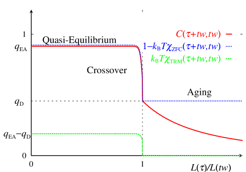
Figure 1: Different asymptotic regimes of the two-time quantities. Here the asymptotic limit $L(t_{\rm w})\to\infty$ is considered with the ratio $x=L(\tau)/L(t_{\rm w})$ being fixed.

We are ready to consider a simple isothermal aging protocol: the temperature is quenched cooling rate at time $t=0$ to a temperature $T$ below its transition temperature $T_{c}$ from above $T_{c}$ and the relaxational dynamics i.e., aging is monitored. The dynamical magnetic susceptibility is generally defined as $\chi(t,t_{\rm w})=N^{-1}\langle M(t)\rangle/h$ where $\langle M(t)\rangle$ is the total magnetization measured at time $t$ and field $h$. In the thermoremanent magnetization (TRM) measurement the field is switched on for a waiting time $t_{\rm w}$ and then cut off: $h(t)=h\theta(t_{\rm w}-t)$. On the other hand, in the ZFC magnetization measurement, the field is switched on after the waiting time: $h(t)=h\theta(t-t_{\rm w})$. We denote the susceptibilities of these protocols as $\chi_{\rm TRM}(t,t_{\rm w})$ and $\chi_{\rm ZFC}(t,t_{\rm w})$. Another important quantity is the magnetic autocorrelation function, $C(t,t_{\rm w})=N^{-1}\langle M(t)M(t_{\rm w})\rangle=N^{-1}\sum_{i}\langle S_{i}(t)S_{i}(t_{\rm w})\rangle$. The last equation follows in the absence of ferromagnetic or anti-ferromagnetic bias.

Within the droplet picture, aging proceeds by coarsening of domain walls FH2 as usual phase ordering processes B94 . Following FH2 , the whole process may be divided into epochs such that the typical size of the domain is $L_{0},aL_{0},a^{2}L_{0},\ldots,a^{n}L_{0},\ldots$. At each epoch, droplets of various sizes up to that of the domain can be thermally activated or polarized by the magnetic field. Importantly the domain wall serves as the frozen-in extended defect for the droplets and reduces their stiffness constant.

In the droplet picture FH2 all dynamical processes, including both the domain growth and droplet excitations in the interior of the domains, are thermally activated processes which yield a logarithmic growth law of the time dependent length scale $L(t)$. In practice, empirical power laws with temperature dependent exponent work as wellKYT ; Uppsala-AC . However, the logarithmic growth law is supported by a recent experiment Uppsala-AC where the effects of critical fluctuations are considered (see alsoHYT ; Saclay-AC ; YHT ; BB ). In the following, we focus on scaling properties of the two time quantities as functions of the dynamical length scale rather than on the growth law itself.

As far as $L(\tau)\leq L(t_{\rm w})$, the autocorrelation function and the ZFC susceptibility are related to the generalized order parameter and linear susceptibility defined in (4) as $C(\tau+t_{\rm w},t_{\rm w})=q(L(\tau),L(t_{\rm w}))$ and $k_{\rm B}T\chi_{\rm ZFC}(\tau+t_{\rm w},t_{\rm w})=1-C(\tau+t_{\rm w},t_{\rm w})$ satisfying the FDT. Especially, the equilibrium correlation and response are obtained by taking the limit $L(t_{\rm w})\to\infty$ with fixed $L(\tau)$. In this special limit one finds FH2 , $C_{\rm eq}(\tau)=q_{\rm EA}+c\tilde{\rho}(0)m^{2}(k_{\rm B}T/\Upsilon)(L(\tau)/L_{0})^{-\theta}$ and

$$\chi_{\rm eq}(\tau)\equiv\lim_{t_{\rm w}\to\infty}\chi_{\rm ZFC}(\tau+t_{\rm w},t_{\rm w})=\chi_{\rm EA}-c\frac{\tilde{\rho}(0)m^{2}}{\Upsilon(L(\tau)/L_{0})^{\theta}}.$$ (9)

In the quasi-equilibrium regime $L(\tau)<L(t_{\rm w})$ waiting time dependence or violation of TTI (Time translational invariance) is present in a weak manner as correction terms to the ideal equilibrium behavior (9). The scaling form of the correction terms can be found using (2) which is relevant for relaxation of AC susceptibilities FH2 ; Uppsala-AC . Actually it allows one to set up numerical extrapolations to obtain the ideal equilibrium behavior KYT ; HYT ; YHT . In the limit $L(t_{\rm w})\to\infty$ with $x=L(\tau)/L(t_{\rm w})<1$ being flexed, we find $C\to q_{\rm EA}$ and $\chi_{\rm ZFC}\to\chi_{\rm EA}$ (see Fig. 1). Much stronger violation of TTI shows up below $q_{\rm EA}$.

In the crossover regime $L(\tau)\sim L(t_{\rm w})$, the anomalously soft droplets as large as the size of the domain $L(t_{\rm w})$ are also needed to be taken into account. From (7) we immediately find, $C(\tau+t_{\rm w},t_{\rm w})|_{L(\tau)\sim L(t_{\rm w})}\sim q_{\rm D}+A(1)\tilde{\rho}(0)m^{2}(k_{\rm B}T/\Upsilon)(L(t_{\rm w})/L_{0})^{-\theta}$ where $q_{\rm D}$ is the novel dynamical order parameter we introduced above. Thus as a function of $x$, there should be a vertical drop from $q_{\rm EA}$ to $q_{\rm D}$ at $x\sim 1$ in the asymptotic limit $L(t_{\rm w})\to\infty$. Correspondingly, the ZFC susceptibility should jump up vertically from $\chi_{\rm EA}$ to $\chi_{\rm D}$ at $x\sim 1$ in the same asymptotic limit (see Fig. 1). Such an abruptness will be absent as functions of $\tau/t_{\rm w}$. Indeed it is well known in experiments Uppsala that the so called relaxation rate $S(t)=d\chi_{\rm ZFC}(\tau+t_{\rm w},t_{\rm w})/d\log(\tau/\tau_{0})$ has a pronounced peak at around $\tau\sim t_{\rm w}$.

In the aging regime $L(\tau)\sim L(t)>L(t_{\rm w})$ we expect,

$$C(t,t_{\rm w})\sim q_{\rm D}\tilde{C}\left(\frac{L(t)}{L(t_{\rm w})}\right).$$ (10)

Here, following Fisher and Huse FH2 , we assume the scaling function $\tilde{C}(x)$ is related to a probability $P_{\rm s}(L(t)/L(t_{\rm w}))$ that a given spin belongs to the same domain at the two different epochs characterized by $L(t)$ and $L(t_{\rm w})$. It satisfies $\tilde{C}(1)=1$ and $\tilde{C}(x)\sim x^{-\lambda}$ at $x\gg 1$ with $\lambda$ being in the range $d/2<\lambda<d$. It should be emphasized that, in contrast to usual domain growth process B94 , we put the dynamical order parameter $q_{\rm D}$ rather than $q_{\rm EA}$ as the amplitude of $C(t,t_{\rm w})$ since we obtained $C(t,t_{\rm w})|_{x\sim 1}\sim q_{\rm D}$ above.

The ZFC susceptibility in the aging regime becomes,

$$\chi_{\rm ZFC}(t,t_{\rm w}) \sim\chi(L(\tau),L(t))$$ (11)

$$+c^{\prime\prime}\int_{L(t_{\rm w})}^{L(t)}\frac{dL}{L}\frac{\tilde{\rho}(0)m^{2}}{\Upsilon(L/L_{0})^{\theta}}\tilde{C}\left(\frac{L(t)}{L}\right)$$

where $c^{\prime\prime}$ is a numerical constant. The first term is due to the response of the droplets equilibrated within the temporal domain of size $L(t)$ (see (4)). The second term represents contributions from the magnetizations (per spin) of order $\tilde{\rho}(0)hm^{2}/\Upsilon(L/L_{0})^{\theta}$ due to droplets as large as $L$ which are induced by the field in the past epochs, say around $t$ with $L(t)=L$, and are depolarized by further domain growth. We also note that this term but with the integration from $L_{0}$ to $L(t_{\rm w})$ yields the TRM susceptibility written as FH2 $\chi_{\rm TRM}(t=\tau+t_{\rm w},t_{\rm w})\sim c_{\rm nst}\tilde{\rho}(0)m^{2}/\Upsilon(L(t_{\rm w})/L_{0})^{-\theta}(L(t)/L(t_{\rm w}))^{-\lambda}$ with $c_{\rm nst}=c^{\prime\prime}\int_{0}^{1}dyy^{-1-\theta+\lambda}>0$. These susceptibilities satisfy the sum rule $\chi_{\rm ZFC}(t,t_{\rm w})+\chi_{\rm TRM}(t,t_{\rm w})=\chi_{\rm ZFC}(t,0)$ which must hold for linear responses.

In the special limit of $t_{\rm w}=0$ we obtain,

$$\chi_{\rm ZFC}(t,0)\sim\chi_{\rm D}-c^{\prime\prime\prime}\frac{\tilde{\rho}(0)m^{2}}{\Upsilon(L(t)/L_{0})^{\theta}}$$ (12)

with $c^{\prime\prime\prime}=A(1)-c_{\rm nst}$. Note that $\chi_{\rm ZFC}(t,0)$ converges to the dynamical susceptibility $\chi_{\rm D}(>\chi_{\rm EA})$ in the limit $t\to\infty$. This implies $\chi_{\rm D}$ is nothing but the field cooled (FC) susceptibility $\chi_{\rm FC}$ cooling rate , while $\chi_{\rm EA}$ is close to what is called the ZFC susceptibility $\chi_{\rm ZFC}$. Thus we expect the well known experimental observation Uppsala ; Saclay $\chi_{\rm FC}>\chi_{\rm ZFC}$ is a dynamical but not a transient phenomenon .

The overall feature of the two time quantities so far discussed is displayed in Fig. 1. Note that a parametric plot of $C$ vs $\chi_{\rm ZFC}$ becomes radically different from the conventional picture BCKM ; FMGPP in which the breaking of FDT and TTI are supposed to happen simultaneously at $(q_{\rm EA},k_{\rm B}T\chi_{\rm EA})$.

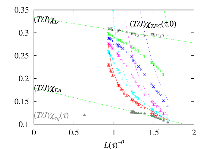
Figure 2: ZFC susceptibilities and spin autocorrelation functions vs $1/L^{\theta}(\tau)$. The symbols are $(T/J)\chi_{\rm ZFC}(\tau+t_{\rm w},t_{\rm w})$ with $t_{\rm w}=0,10,10^{2},10^{3},10^{4},10^{5}$ MC step from the top to the bottom. The maximum time separation is $\tau=10^{5}$ MC step. The curves with lines are corresponding $1-C(\tau+t_{\rm w},t_{\rm w})$. The data of $(T/J)\chi_{\rm eq}(\tau)$ (filled triangle) is shown at the bottom.

Finally let us briefly discuss some numerical results concerning our scenario. We performed Monte Carlo (MC) simulations of isothermal aging of a 4 dimensional EA spin-glass model (size $24^{4}$)with $\pm J$ interactions ($T_{c}=2.0J$, with $k_{\rm B}=1$ here and hereafter) starting from random initial conditions. A set of data of $1-C(\tau+t_{\rm w},t_{\rm w})$ and $(T/J)\chi_{\rm ZFC}(\tau+t_{\rm w},t_{\rm w})$ at $T/J=0.8$ is plotted against $L(\tau)^{-\theta}$ in Fig. 2. The field of strength $h/J=0.1$ was used and the linearity of the responses was checked by the sum rule, $\chi_{\rm ZFC}(t,t_{\rm w})+\chi_{\rm TRM}(t,t_{\rm w})=\chi_{\rm ZFC}(t,0)$. We used $\theta=0.82$ obtained by a defect free-energy analysis KH . For the growth law $L(t)$, we used the result of an independent measurement of the growth of domain HYT ; YHT . As explained in KYT ; HYT ; YHT the analysis of the quasi-equilibrium yields the equilibrium limit curve shown at the bottom of the figure (See HYT ). It follows the scaling form (9) pointing toward $(T/J)\chi_{\rm EA}\simeq 0.18$. The other extreme $\chi_{\rm ZFC}(\tau,0)$ also becomes linear in this plot as expected in (12) pointing toward $(T/J)\chi_{\rm D}\simeq 0.34$ well above $\chi_{\rm EA}$. Apparently FDT ($(T/J)\chi=1-C$) is well satisfied at small $\tau$ and broken at large $\tau$. Interestingly enough, the break points of the FDT move further away from $(T/J)\chi_{\rm eq}(\tau)$ suggesting the separation of the breaking of FDT and TTI as we anticipated. Such a feature has not been reported in previous numerical studies FDT-MC .

We also confirmed most of other scaling ansatz of the two time quantities within the 4D EA model which will be presented elsewhere YHT . It will be certainly interesting to test our scenario by experiments such as noise measurements HO and further numerical simulations.

- (1) “Spin Glasses and Random Fields”, A.P. Young Editor, (World Scientific, 1998).
- (2) P. Nordblad and P. Svedlindh, in APY-review .
- (3) E. Vincent, J. Hamman, M. Ocio, J. -P. Bouchaud and L. F. Cuglinadolo, in Proceeding of the Sitges Conference on Glass Systems, E. Rubi Editor, (Springer, 1996).
- (4) H. Rieger, in Annual Review of Computational Physics II, edited by D. Stauffer (World Scientific, 1995).
- (5) J. -P. Bouchaud, L. F. Cugliandolo, J. Kurchan and M. Mézard in APY-review .
- (6) L. F. Cugliandolo and J. Kurchan, Phys. Rev. Lett. 71, 173 (1993); J. Phys. A 27, 5749 (1994); S. Franz and M. Mézard, Europhys. Lett. 26, 209 (1994); Physica A 209, 1 (1994). L. F. Cugliandolo and P. Le Doussal, Phys. Rev. E 53, 1525 (1996).
- (7) L. F. Cugliandolo, J. Kurchan and L. Peliti, Phys. Rev. E 55, 3898 (1997).
- (8) A. J. Bray and M. A. Moore, Phys. Rev. Lett. 58, 57 (1987).
- (9) D. S. Fisher and D. A. Huse, Phys. Rev. B38, 386 (1988).
- (10) D. S. Fisher and D. A. Huse, Phys. Rev. B38, 373 (1988).
- (11) J. Houdayer and O. C. Martin, Euro. Phys. Lett. 49, 794 (2000); F. Krazakala and O. C. Martin, Phys. Rev. Lett. 85, 3013 (2000); M. Palassini and A. P. Young, Phys. Rev. Lett. 85, 3017 (2000).
- (12) C. M. Newman and D. L. Stein, Phys. Rev. E 57, 1356 (1998); Phys. Rev. Lett. 87, 077201 (2001).
- (13) A. Middleton, Phys. Rev. Lett. 83, 1672 (1999).
- (14) T. Komori, H. Yoshino and H. Takayama, J. Phys. Soc. Jpn. 68, 3387 (1999); J. Phys. Soc. Jpn. 69, 1192 (2000).
- (15) H. G. Katzgraber, M. Palassini, and A. P. Young, Phys. Rev. B 63, 184422 (2001) and references there in.
- (16) Infinitely fast cooling is considered so that TRM becomes the same as isothermal remanent magnetization (IRM).
- (17) Unfortunately the ambiguity of the width is unavoidable within the independent droplet model.
- (18) A. J. Bray, Adv. Phys. 43, 357 (1994).
- (19) P. E. Jönsson, H. Yoshino, P. Nordblad, H. Aruga Katori and A. Ito, cond-mat/0112389.
- (20) V. Dupis, E. Vincent, J.-P Bouchaud, J. Hammann, A, Ito and H. A. Katori., Phys. Rev. B 64 174204 (2001).
- (21) K. Hukushima, H. Yoshino and H. Takayama, Prog. Theor. Phys. Supp. 138, 568 (2000), cond-mat/9910414.
- (22) H. Yoshino, K. Hukushima and H. Takayama, cond-mat/0202110.
- (23) L. Bertheir and J.-P. Bouchaud, cond-mat/0202069.
- (24) S. Franz, M. Mézard, G. Parisi, L. Peliti, Phys. Rev. Lett. 81, 1758 (1998).
- (25) K. Hukushima, Phys. Rev. E 60, 3606 (1999).
- (26) S. Franz and H. Rieger, J. Stat. Phys. 79, 749 (1995); G. Parisi, F. Ricci-Tersenghi and J. J. Ruiz-Lorenzo, J. Phys. A 29, 7943 (1996); E. Marinari, G. Parisi, F. Ricci-Tersenghi and J. J. Ruiz-Lorenzo, J. Phys. A 31, 2611 (1998).
- (27) D. Hérisson and M. Ocio, cond-mat/0112378.