Competition Among Companies: Coexistence and Extinction

Abstract

We study a spatially homogeneous model of a market where several agents or companies compete for a wealth resource. In analogy with ecological systems the simplest case of such models shows a kind of “competitive exclusion” principle. However, the inclusion of terms corresponding for instance to “company efficiency” or to (ecological) “intracompetition” shows that, if the associated parameter overcome certain threshold values, the meaning of “strong” and “weak” companies should be redefined. Also, by adequately adjusting such a parameter, a company can induce the ”extinction” of one or more of its competitors.

I Introduction

During the last few years we have witnessed a wealth of work on the application of methods of statistical physics to the study of economic problems configuring what some authors called econophysics uno ; dos ; tres ; cuatro . Within this framework a great deal of effort was dedicated to the analysis of economic data ranging from stock exchange fluctuations uno , production models, size distribution of companies, the appearance of money, effects of control on the market to market critical properties cinco . Another problem that attracted enormous interest was the origin of power (Paretto) laws, and lognormal distribution with power law tails, for the income of individuals, wealth distribution, debt of bankrupt companies SS . An interesting source of several mathematical descriptions and models used in economical and sociological contexts can be found in haag .

Here, our interest is the study, in a deterministic way, of aspects of the competition and coexistence of agents or companies in a common market. We present a simple “toy” model describing, in analogy to some ecological problems, a situation of competition among several companies. Within a “Malthusian-like” model we analyze the effect of a kind of intracompetitive contribution on the possibility of companies coexistence in a certain market, and the changing leadership role (measure through some wealth parameter) between, according to the standard ecological definition, “strong” and “weak” companies.

According to ecological studies, starting with Volterra’s first results on the mathematical theory of competition vol , the problem of competition and coexistence between species has been analyzed and resumed within the Competitive Exclusion Principle (or Ecological Theorem), that states: $N$ species that compete for $n(<N)$ food resources, cannot coexist mur . Several aspects of this problem have been analyzed by different authors, emphasizing, for instance, the conflict between the need to forage and the need to avoid competition; effects of diffusion-mediated persistence. Generally, the system describing competition between species can be represented by a set of $N$ differential equations for the species and $n$ for the resources. As an example, with only one food resource we find only two stable stationary solutions: the trivial one (extinction of all he species), and that corresponding to the survival of only one species, the “strongest” one. There are also studies of the problem related to the possibility of coexistence in the form of wave–like solutions sch ; wkvh .

Here we adapt the model used in Refs.sch ; wkvh for the case of a homogeneous competitive market with a unique wealth resource and several firms. In the next Section we introduce the model and some particular, instructive, solutions. Due to the difficulties of finding analytical solutions for the general case, in Section III we focus on a representative system with a small number (here 4) of firms, and analyze its behavior by numerical methods. In the last Section we draw some conclusions.

II The Model

We start describing the model we use, which is related to the one used in Refs.sch ; wkvh for the study of coexistence in an ecological framework in the form of wave–like solutions. Such a model has been adapted to the problem of competition of $N$ agents or companies for a unique common wealth resource. We indicate with $n_{j}$ the “size” or wealth-parameter representing the welfare of the $j$-company ($j=1,...,N$) and with $M$ the total amount of “wealth”. The set of differential equations that we use to describe the behavior (for the homogeneous case) of such a complex system includes a “Malthusian-like” birth-death equation mal for each company ($\beta_{j}\,M(t)\,n_{j}(t)\,\,$ corresponding to benefits coming from the wealth’s share and $\,\,-\alpha_{j}\,n_{j}(t)\,\,$ for the “standard” losses–or costs– of the $j$-th company). We also include a contribution that corresponds, in ecological language, to taking into account the existence of some kind of intracompetition, that is if the $j$-th the company is alone and can get all the wealth $M$, it can only grow up to a maximum bounded size, a behavior that can be modelled by a Verhulst-like term mur . This takes into account the in ecological contexts so called carrying capacity of the economic environment ccap ; yad . In economic terms it could correspond to an increase of the company efficiency, for instance, through the reduction of operative internal costs, improved management, avoiding of competition between different branches of the same firm, instrumentation of new technologies, etc.

In addition, instead of assuming a constant finite wealth resource as in the so called “Total Wealth Conserved model” piav , we consider that $M$ has its own dynamics. For the equation for $M$, the economic wealth accessible to the companies that, in order to simplify this initial analysis we assume is unique, we also consider a “Malthusian-like” behavior including: its production (new resources and technologies, harvest and grain production, etc) that we assume has a constant rate $Q$, and its disappearance due to: (a) natural degradation or rotting of crops, technologies becoming old, some resources being exhausted, that we assume has a rate proportional to the total wealth amount $-GM$ (only a certain portion of $M$ disappears), (b) the share of each company given by $-\beta_{k}\,n_{k}(t)\,M(t)$.

The set of equations is ($j=1,...,N$)

$$\frac{d}{dt}n_{j}(t) = [\beta_{j}\,M(t)-\alpha_{j}]\,n_{j}(t)-\gamma_{j}\frac{n_{j}^{2}}{M}$$

$$\frac{d}{dt}M(t) = Q(t)-[G+\sum\beta_{k}\,n_{k}(t)]\,M(t).$$ (1)

Similarly to what was discussed in wkvh for the case of only two species, we can here define a hierarchy from the “strongest” (largest ratio between wealth share and standard losses, i.e. largest $\frac{\beta_{i}}{\alpha_{i}}$) to the “weakest” (smallest ratio) companies. Assuming the following hierarchical order

$$\frac{\beta_{1}}{\alpha_{1}}>\frac{\beta_{2}}{\alpha_{2}}>...>\frac{\beta_{N}}{\alpha_{N}},$$ (2)

we have that $n_{1}$ is the strongest company while $n_{N}$ is the weakest one. It is worth noting in passing that Eqs.(II) resembles the form of multimode laser systems lasers , making it possible to transfer some results from one system to the other.

The stationary solutions results from taking $\frac{d}{dt}M=0$ and $\frac{d}{dt}n_{j}=0$ ($j=1,...,N$). We found

$$M_{s} = \frac{Q(t)}{G+\sum\beta_{k}\,n_{k}^{s}}$$ (3)

$$0 = \left([\beta_{j}\,M_{s}-\alpha_{j}]-\gamma_{j}\frac{n_{j}^{s}}{M_{s}}\right)\,n_{j}^{s}.$$ (4)

The last equation implies one of two possibilities

$$n_{j}^{s}=0,\,\,\,\,\,\,\,\mbox{or}\,\,\,\,\,\,\,n_{j}^{s}=\frac{[\beta_{j}\,M_{s}-\alpha_{j}]\,M_{s}}{\gamma_{j}}.$$ (5)

It is clear that for large $N$, to find the solution of this system is not easy. In order to fix ideas we consider the simplified case where, instead of the above indicated hierarchy, we have that all companies are equivalent, that is

$$\beta_{j}=\beta,\,\,\,\,\alpha_{j}=\alpha,\,\,\,\,\gamma_{j}=\gamma,$$

implying

$$n_{j}^{s}=n_{s}\,\,\,\,\,\,\ \forall\,j.$$

In this case we have

$$n_{s}=\frac{[\beta\,Q-(\alpha/Q)(G+N\beta n_{s})]\,Q^{2}}{\gamma(G+N\beta n_{s})^{2}},$$ (6)

that can be rewritten as

$$-\frac{\gamma N^{2}\beta}{Q^{2}}n_{s}^{3}-\frac{2\gamma GN\beta}{Q^{2}}n_{s}^{2}-\left(\frac{\alpha\beta N}{Q}+\frac{\gamma G^{2}}{Q^{2}}\right)n_{s}+(\beta-\frac{\alpha G}{Q})=0.$$ (7)

It is possible to find under which conditions at least one solution of Eq. (7) is real. However, it is more instructive to look for the behavior at small $n_{s}$ ($n_{s}\sim 0$) as all the coefficients of $n_{s}^{\nu}$ with $\nu>0$ are negative. Hence, we can easily obtain that a solution, given by

$$n_{s}\approx\frac{\beta Q^{2}-\alpha GQ}{\alpha\beta NQ+\gamma G^{2}},$$

exists (is positive) if $\beta Q>\alpha G.$ In this case, as one of the associated eigenvalues is zero, a linear stability analysis does not give a clear information about the stability of the solution and it is necessary to resort to a more refined analysis.

Another instructive case is to consider

$$\frac{\beta_{1}}{\alpha_{1}}>\frac{\beta_{2}}{\alpha_{2}}=...=\frac{\beta_{N}}{\alpha_{N}}.$$

Here we reduce to essentially the same situation studied in sch ; wkvh . In particular, it is coincident with the situation studied in KW , but now having an “effective” weak species given by $(N-1)n_{j}$, $j=2,N$. As in KW , and as discussed in detail latter for the case of several firms, it is possible to find a coexistence region when $\gamma_{1}$ overcomes some threshold value. In this case a linear stability analysis shows a change in the stability of these solutions.

As a general analytical study of our system even for $N$ not too large is far beyond our interest, in the next section we focus on a numerical approach for a case with a small, however representative, value of $N$ analyzing some relevant situations.

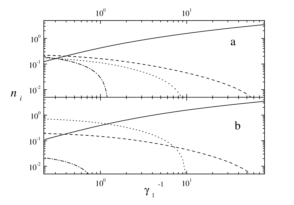
Figure 1: Asymptotic values of $n_{i}$ for different values of $\gamma_{1}^{-1}$. In both cases $\rho_{1}=5$, $\rho_{2}=2.5$, $\rho_{3}=1.5$, $\rho_{4}=1$. Full line: Species 1; Dash line: Species 2; Dotted line: Species 3; Dash-dotted line: Species 4. In a) $\gamma_{2}=1$, $\gamma_{3}=0.5$ and $\gamma_{4}=0.1$, in b) $\gamma_{2}=1$, $\gamma_{3}=0.1$ and $\gamma_{4}=0.5$.

III Numerical Results

As indicated before, here we focus in a case with $N$ small (in fact $N=4$) that shows all the relevant aspects we can expect in the large $N$ situation. Defining the ratio $\rho_{i}=\frac{\beta_{i}}{\alpha_{i}}$ we consider several situations:
a) when the different companies are in hierarchical order, that is $\rho_{1}>\rho_{2}>\rho_{3}>\rho_{4}$;
b) when we have $\rho_{1}>\rho_{2}=\rho_{3}=\rho_{4}$;
c) when $\rho_{1}=\rho_{2}>\rho_{3}=\rho_{4}$.

Among all the possible scenarios we have chosen those showing regions of coexistence of all the species, thus in case (a) we investigate the situation with fixed $\gamma_{j}$, with $j=2,3,4$ and varying $\gamma_{1}$. That allows us to have a control parameter, but we recall that the choice is arbitrary. In this case the usual strong and weak concepts make us consider the species 1 as the strongest and the 4 as the weakest. With the inclusion of the new term we find not only the possibility of coexistence but also that the original hierarchical order can be permuted several times as the parameter values are varied. Thus, we find that the ranking of companies suffers many changes, with companies interchanging roles several times. Some examples of this case are shown in Fig.1. Besides these new features we observe the classical extinction of companies as predicted by the exclusion theorem. In all the cases the extinction occurs by one species at a time. Figure 1 shows two typical results for the stationary values reached by $n_{j}$ as function of $\gamma_{1}^{-1}$. It is apparent that according to the different values, the relative status of each company can change and even reversed with several crossing among them. In this figure $\gamma_{1}$ varies continuously from 10 to 0. The ratios $\rho_{i}=\frac{\beta_{i}}{\alpha_{i}}$ are $\rho_{1}=5$, $\rho_{2}=2.5$, $\rho_{3}=1.5$, $\rho_{4}=1$. In Fig.1a we have $\gamma_{2}=1$, $\gamma_{3}=0.5$ and $\gamma_{4}=0.1$, while in Fig 1.b $\gamma_{2}=1$, $\gamma_{3}=0.1$ and $\gamma_{4}=0.5$.

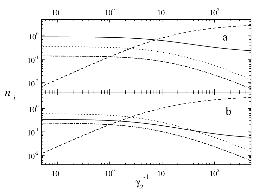
Figure 2: As in Figure 1 with $\rho_{1}=4$, $\rho_{2}=\rho_{3}=\rho_{4}=2$ and a) $\gamma_{1}=.25$, $\gamma_{3}=0.5$ and $\gamma_{4}=0.1$, in b) $\gamma_{1}=1$, $\gamma_{3}=0.5$ and $\gamma_{4}=0.1$.

For the case (b) above, we considered as our variable $\gamma_{2}$. In this case we have one strong species with $\rho_{1}=4$, and three similar species, $\rho_{2}=\rho_{3}=\rho_{4}=2$, that could coexist if there was not a strongest one. We want to note that though $\rho_{2}=\rho_{3}=\rho_{4}$ the same is not true for $\alpha$ and $\beta$ values. Once again, we observe coexistence between species and a reorganization of the company or agents ranking, not accordingly to the original concept of strength but depending of the values of $\gamma_{i}$. The coexistence is achieved within certain parameter region. The extinction is gradual and governed mainly by $\gamma$ values. The results are shown in Fig. 2, where again we depict the stationary values of $n_{j}$ as functions of $\gamma_{x}^{-1}$. In Fig 2.a we have $\gamma_{1}=0.25$, $\gamma_{3}=0.5$, $\gamma_{4}=0.1$, while in Fig 2.b $\gamma_{1}=1.$, $\gamma_{3}=0.5$, $\gamma_{4}=0.1$. It is apparent that the most relevant parameter when considering competition is the value of $\gamma_{i}$. When species are equally strong or weak, we observe that different stationary density levels are reached according to $\gamma_{i}$. If $\gamma_{i}$ is of the same order the coexistence is granted. On the contrary, a species with a high $\gamma_{i}$ will not survive even if competing with similar species. As an additional feature we observe that a usual strong species $j$ will not survive even if competing with weaker species if $\gamma_{j}$ is much higher than that of the other species.

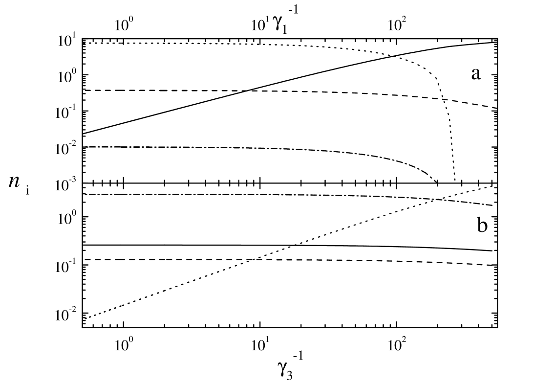
Figure 3: As in Figure 1 with $\rho_{1}=\rho_{2}=4$, $\rho_{3}=\rho_{4}=2$ and a)$\gamma_{2}=0.25$, $\gamma_{3}=10^{-3}$ and $\gamma_{4}=1.5$, in b) $\gamma_{1}=0.5$, $\gamma_{2}=0.5$ and $\gamma_{4}=0.01$

In case (c) we considered two situations: a first one varying $\gamma_{1}$; and a second varying $\gamma_{3}$. The results are shown in Fig. 3, where again we depict the stationary values of $n_{j}$ as functions of $\gamma_{1}^{-1}$ and $\gamma_{3}^{-1}$ respectively. In both cases 3 $\rho_{1}=\rho_{2}=4$, $\rho_{3}=\rho_{4}=2$, while in a) $\gamma_{2}=0.25$, $\gamma_{3}=0.001$, $\gamma_{4}=1.5$ and in b)$\gamma_{1}=0.5$, $\gamma_{2}=1.5$, $\gamma_{4}=0.01$ . We confirm that the coexistence can be achieved for proper $\gamma$ values. At the same time we observe that the usual concept of strongest species cannot be applied as in both previous cases, species 2, one of the strongest if $\gamma_{i}$ were zero remains as the weakest species due to a high $\gamma_{2}$ value.

IV Conclusions

The results shown above indicates how the study of simplified models could help in the understanding of the role played by $\gamma$, an internal company parameter, associated to the company efficiency, in situations where the complexity of the economic reality makes very hard to obtain a complete model. In our case, the model so far studied could give some hints on the behavior of systems of companies in competition and the possibility of coexistence and the way that one company can use to “eliminate” the competing ones adopting a policy tending to adequately change its $\gamma$. Here we have analyzed the effect of explicitly including the carrying capacity of the environment within our toy model for describing the coexistence of species in competition. The results put in evidence the role played by the term associated to $\gamma$ in the possibility of coexistence. We recall that in the absence of such term the exclusion principle is valid and only the species (one or more) with the highest $\rho$ survive. It is also this term that, within certain parameter region, governs the company or agents ranking. A model written in the same terms can clearly also be applicable to ecological situations. But in this case, rather than a deterministic control of $\gamma$, some fluctuations or cyclic changes in this parameter should be considered. This is the subject of a work of us in progress.

Acknowledgements: Partial support from CONICET and ANPCyT, both Argentina agencies, as well as to Fundación Antorchas, are greatly acknowledged. HSW wants to thank to Iberdrola S.A., Spain, for an award within the Iberdrola Visiting Professor Program in Science and Technology, and to the IMEDEA and Universitat de les Illes Balears, Palma de Mallorca, Spain, for the kind hospitality extended to him.

References

- (1) R. N. Mantegna and H. E. Stanley, An Introduction to Econophysics: Correlations and Complexity in Finance, (Cambridge U.P., Cambridge, 1999).
- (2) Proc. Int. Workshop on Econophysics and Statistical Finance, Ed. R. Mantegna, Physica A 269#1 (1999); Economic Dynamics from the Physics Point of View, Eds. F. Schweitzer and D. Helbing, Physica A 287 # 3-4 (2000); Proc. NATO ARW Applications of Physics in Economic Modelling, Eds. J.P. Bouchaud, M. Marsili, B,M, Roehner and F. Slamina, Physica A 299 # 1-2(2001).
- (3) J.P. Bouchaud and M. Potters, Theory of Financial Risk, (Cambridge U.P., Cambridge, 2000).
- (4) W.B. Arthur, S. Durlauf and D. Lane, Eds., The Economy as a Complex System II, (Addison-Wesley, Redwood City, 1997).
- (5) P. Bak, K. Chen, J. A. Scheinkman and M. Woodford, Ricerce Economiche 47, 3 (1993); M.H.R. Stanley, et al., Scaling behaviour in the growth of companies, Nature 379, 804 (1996); R.Donangelo and K. Sneppen, Physica A 276, 272 (2000); G. Cuniberti, A. Valleriani and J.L. Vega, Quantitative Finance 1, 332 (2001); B.B. Mandelbrot, Fractal and Scaling in Finance (Springer, New York, 1997).
- (6) S. Solomon and M. Levy, Int.J. Mod. Phys. C 7, 745 (1996), S. Solomon, in Computational Finance ’97, A-P.N. Refenes, A.N. Burgess and J.E. Moody (Eds.) (Kluwe Ac.Pub., Dordrecht, 1998); H. Aoyama, et al., Fractals 8, 293-300 (2000); J-P. Bouchaud and M. Mèzard, Physica A 282, 536-545 (2000).
- (7) G. Haag, U. Müller and K.G. Troitzsch, Eds, Economic Evolution and Demographic Change: Formal Models in Social Science, (Springer-Verlag, Berlin, 1992).
- (8) Volterra, V., R. Comitato Talassografico Italiano, Memoria 131, pp 1-142 (1927).
- (9) Murray, J. D., Mathematical biology, Springer–Verlag, 1989.
- (10) Mikhailov, A. S., Phys. Lett. 73A, 143 (1979); Mikhailov, A. S., Z. Physik B 41, 277 (1981); Mikhailov, A. S., Phys. Rep. 184, 308 (1989).
- (11) C. Schat, M. Kuperman and H.S. Wio, Math. Biosciences 131, 205 (1996).
- (12) M. Kuperman, M., B. von Haeften and H.S. Wio, Quantum Mechanical Analogy for Solving a Competitive Coexistence Model in Ecology, ICTP Report IC/94/186 (1994); M. Kuperman, B. von Haeften and H.S. Wio, Bull.Math.Biology 58, 1001-1018 (1996); H.S. Wio, M. Kuperman, B.von Haeften, M. Bellini and R. Deza, Competitive coexistence in biological systems: exact analytical results through a quantum mechanical analogy, in Instabilities and Nonequilibrium Structures V, E. Tirapegui y W. Zeller Eds.(Kluwer, 1995).
- (13) Malthus, T. R., An essay on the principle of population, 1798, Penguin Books, 1970.
- (14) Freedman, H.I.; Deterministic Mathematical Models in Population Ecology, (M.Dekker, N.Y., 1980); chapters 7 and 8.
- (15) P.Yodzis, Introduction to Theoretical Ecology, (Harper & Row, N.Y., 1989), Chapter 5.
- (16) S. Pianegonda, J.R.Iglesias, G. Abramson and J.L. Vega, Wealth redistribution with finite resources, nlin.AO/0109015, (2001).
- (17) See for instance G.P.Agrawal and N.K.Dutta, Long-Wavelength Semiconductor Laser (Van Nostrand Reinhold, New York, 1986).
- (18) H.S. Wio and M.N. Kuperman, A phase transition induced by the struggle for life in a competitive coexistence model in ecology, ICTP Report , (1994).