One-dimensional non-interacting fermions in harmonic confinement: equilibrium and dynamical properties

Abstract

We consider a system of one-dimensional non-interacting fermions in external harmonic confinement. Using an efficient Green’s function method we evaluate the exact profiles and the pair correlation function, showing a direct signature of the Fermi statistics and of the single quantum-level occupancy. We also study the dynamical properties of the gas, obtaining the spectrum both in the collisionless and in the collisional regime. Our results apply as well to describe a one-dimensional Bose gas with point-like hard-core interactions.

1 Introduction

Atomic Fermi vapours have been cooled down to degeneracy in several experiments on ultra-cold atoms of ⁶Li and ⁴⁰K [1, 2, 3], using techniques similar to those employed to obtain Bose-Einstein condensation [4]. At very low temperatures collisions between atoms are essentially in the $s$-wave channel; however, all even-channel collisions are forbidden for spin-polarized fermions by the Pauli exclusion principle. Since dipolar interactions are also negligible, the Fermi gas can be considered as non-interacting. In the experiments the atoms are trapped by magnetic or optical potentials, providing a confinement which can be well approximated as harmonic. The geometry of the trapping potential can be very anisotropic, thus allowing to reach quasi-1D or quasi-2D situations [5].

We focus here on the quasi-1D geometry, which is the case of the Paris experiment [3] and is relevant for experiments on atom lasers and atomic waveguides. The 1D gas of non-interacting fermions serves also as a model for describing the 1D Bose gas with hard-core point-like interactions (Tonks gas, [6]). Indeed, it was demonstrated by Girardeau that there exists an exact mapping between the bosonic and the fermionc many-body wave functions, $\Psi_{B}=|\Psi_{F}|$, valid also in the time domain [7, 8]. The Tonks gas limit corresponds to the case of total reflection in a two-atom collision [9], and the interactions in 1D mimic the role of the Fermi statistics.

In this paper we present some results for the exact equilibrium profiles and for the dynamical properties of a 1D Fermi gas in harmonic confinement. In Sec. 2 we illustrate the role of quantum statistics on the particle and kinetic-energy density profiles, and we investigate how the Pauli principle influences the pair correlation function. In Sec. 3 we evaluate the spectrum of the gas both in the collisionless and in the collisional regime. In addition, we relate the result for the frequency of the quadrupole mode to a scaling property of the Hamiltonian used in the long-wavelength limit. Finally, Sec. 4 offers a summary and some concluding remarks.

2 Equilibrium properties

We consider a system of $N$ non-interacting Fermi particles confined in an external potential which is very tight in two spatial directions. We assume that the gas is in a quasi-1D situation where the transverse degrees of freedom are frozen, that is, the chemical potential is much smaller than the level spacing in the transverse direction. In this case the transverse wave function is the ground state one, which will factorize out from all the following calculations. We can thus focus only on the axial coordinate $x$ and define the external confinement along $x$ given by a real potential $V_{ext}(x)$. For the sake of simplicity we will assume that the eigenfunctions $\psi_{i}(x)$ are real [10].

The equilibrium properties of the gas can be expressed in terms of the longitudinal one-body density matrix, which at zero temperature reads

$$\rho^{(l)}(x,x^{\prime})=\sum_{i=1}^{N}\psi_{i}(x)\psi_{i}(x^{\prime}).$$ (1)

In the following we will give several examples of calculations of the exact spatial profiles obtained as the moments of the density matrix, and we will evaluate also the longitudinal pair distribution function.

2.1 Density profiles

The zeroth moment of the one-body density matrix yields the equilibrium density profile $n(x)$

$$n(x)=\rho^{(l)}(x,x^{\prime})|_{x^{\prime}=x}=\sum_{i}\langle\psi_{i}\,|\delta(x-x_{i})|\,\psi_{i}\rangle,$$ (2)

where $x_{i}$ are the positions of the fermions and $|\,\psi_{i}\rangle$ are the eigenstates of the Hamiltonian in the coordinate representation. We have shown [11] that $n(x)$ can be written in terms of the Green’s function in coordinate space, $\hat{G}(x)=(x-\hat{x}+i\varepsilon)^{-1}$, which is a function of the position operator $\hat{x}$:

$$n(x)=-\frac{1}{\pi}\lim_{\varepsilon\rightarrow 0^{+}}{\rm Im}\,\sum_{i=1}^{N}\langle\psi_{i}\,|\hat{G}(x)|\,\psi_{i}\rangle\;.$$ (3)

This equation expresses the density profile as the trace of the operator $\hat{G}(x)$ on the first $N$ quantum states (${\rm Tr}_{N}$). Using the relation between the partial trace ${\rm Tr}_{N}$ of a generic matrix $Q$ and the determinant of the inverse matrix $Q^{-1}$,

$${\rm Tr}_{N}Q=\partial[\ln\det(Q^{-1}+\lambda{\mathbb{I}}_{N})]/\partial\lambda|_{\lambda=0},$$ (4)

we obtain

$$n(x)=-\frac{1}{\pi}\lim_{\varepsilon\rightarrow 0^{+}}{\rm Im}\,\frac{\partial}{\partial\lambda}[\ln\det(x+i\varepsilon-\hat{x}-\lambda{\mathbb{I}}_{N})]_{\lambda=0}\;.$$ (5)

This alternative expression for the density profile is very practical for performing numerical calculations in the case of harmonic confinement, $V_{ext}(x)=m\omega_{ho}^{2}x^{2}/2$. For this specific potential the representation for both the position and the momentum operators on the basis $\psi_{i}$ of the eigenstates of the harmonic oscillator is a tridiagonal matrix. Thus the operator $x+i\varepsilon-\lambda{\mathbb{I}}_{N}$ is tridiagonal: the determinant of such a matrix can be evaluated recursively through a renormalization procedure [11, 12].

The numerical results for the particle density profiles are shown in Fig. 1 at various number of fermions, as compared with the predictions of the local-density approximation: the latter neglects the shell structure and the spill-out from the classical border. Because of the symmetry between position $\hat{x}$ and momentum $\hat{p}$ in the harmonic-oscillator Hamiltonian, the momentum distribution has exactly the same behaviour as the particle density illustrated in Fig. 1.

On account of the mapping with the Tonks gas the particle density profile of $N$ noninteracting fermions in the 1D harmonic trap is identical to that of $N$ bosons with hard-core interactions in the same external potential, while the momentum distribution for such a system has a sharp peak at small wavevectors [13].

2.2 Kinetic energy and momentum flux densities

The first moment and all the other odd moments of the one body density matrix are zero because of the reality of the wave functions. For higher even moments several definitions are avaible in the literature (for a review see e.g. Ref. [14]); these can be expressed again in terms of $\hat{G}(x)$ [12]. In particular, we shall concentrate on the quantity

$$P_{n}(x) = (-i)^{n}\left[\frac{\partial^{n}}{\partial{x^{\prime}}^{n}}\rho^{(l)}(x,x^{\prime})\right]_{x^{\prime}=x}$$ (6)

$$= -\frac{1}{\pi}\lim_{\varepsilon\rightarrow 0^{+}}{\rm Im}\,\sum_{i=1}^{N}\langle\psi_{i}\,|\hat{G}(x)\hat{p}^{n}|\,\psi_{i}\rangle\;$$

and on its symmetrized form

$$S_{n}(x) = (-i)^{n}\left[\frac{\partial^{n}}{\partial r^{n}}\rho^{(l)}(x+r/2,x-r/2)\right]_{r=0}$$ (9)

$$= -\frac{1}{\pi}\frac{1}{2^{n}}\sum_{\sigma=0}^{n}\left(\begin{array}[]{c}n\\ \sigma\\ \end{array}\right)\lim_{\varepsilon\rightarrow 0^{+}}{\rm Im}\,\sum_{i=1}^{N}\langle\psi_{i}\,|\hat{p}^{\sigma}\hat{G}(x)\hat{p}^{n-\sigma}|\,\psi_{i}\rangle\;.$$

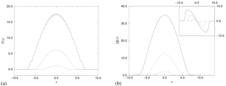
Here we have set $\hbar=1$ and $m=1$. For $n=2$ these definitions give rise respectively to twice the local kinetic energy $T(x)$ [Eq. (6)] and to the momentum flux density $\Pi(x)$ [Eq. (9)]. Although the semiclassical limits and the integrals of these two functions coincide, in the quantum limit these are different functions: the kinetic energy density is invoked in density-functional theory, while the momentum flux density appears in the equations of generalized hydrodynamics.

The same method which was used in Sec. 2.1 to express the density profile in terms of the determinant of the inverse of the Green’s function operator can be extended to deal with the operators of the form $\hat{p}^{\sigma}\hat{G}(x)\hat{p}^{n-\sigma}$ [12]. Again, for low values of $n$ one is reduced to evaluate with recursive methods the determinant of sparse matrices, which are always tridiagonal in the tails.

The kinetic energy and the momentum flux densities obtained with this procedure are shown in Fig. 2 for various number of fermions in 1D harmonic confinement. Oscillations along the profile and negative tails are found in the kinetic energy density, while a smooth positive profile is obtained for the momentum flux density (which however shows oscillations in its first derivative, see the inset of Fig. 2). Other properties of these curves are that the tails of the momentum flux density profile can be expressed analytically in terms of the von Weiszäcker surface energy $(\hbar^{2}/8m)|\nabla n(x)|^{2}/n(x)$ [15], and that an approximate form of the kinetic energy density can be found using the exact density profile in the local-density expression $T(x)=\pi^{2}\hbar^{2}[n(x)]^{3}/6m$ [16].

2.3 Pair distribution function

Higher order correlations are described in the equal-times pair distribution function. We focus here on how the Pauli exclusion principle is reflected in the pair distribution function of a gas of $N$ noninteracting fermions in harmonic confinement. The same results apply to a 1D Bose gas with hard-core interactions, since the boson-fermion mapping holds for the pair distribution function [13].

The longitudinal pair distribution function of a quasi-1D Fermi gas is defined as

$$\rho^{(l)}_{2}(x_{1},x_{2})=n(x_{1})n(x_{2})-F(x_{1},x_{2}),$$ (10)

where the function $F(x_{1},x_{2})$ is given by

$$F(x_{1},x_{2})=\sum_{i,j=1}^{N}\phi_{i}^{*}(x_{1})\phi_{j}(x_{1})\phi^{*}_{j}(x_{2})\phi_{i}(x_{2})$$ (11)

This function can be calculated by an extension of the Green’s function method used in the previous sections to evaluate particle, kinetic energy and momentum flux densities [17]. We first rewrite Eq. (11) in terms of the Green’s function $\hat{G}(x)$,

$$F(x_{1},x_{2})=\frac{1}{\pi^{2}}\lim_{\varepsilon\rightarrow 0^{+}}\sum_{i,j=1}^{N}{\rm Im}\langle\psi_{i}|\hat{G}(x_{1})|\psi_{j}\rangle\,{\rm Im}\langle\psi_{j}|\hat{G}(x_{2})|\psi_{i}\rangle\;;$$ (12)

we then use the property ${\rm Im}A\cdot{\rm Im}B=(1/2)[{\rm Re}(A\cdot B^{*})-{\rm Re}(A\cdot B)]$ to obtain the final expression

$$F(x_{1},x_{2})=\frac{1}{2\pi^{2}}\lim_{\varepsilon\rightarrow 0^{+}}\left\{{\rm Re}{\rm Tr}\left[\hat{G}_{N}(x_{1})\cdot\hat{G}^{*}_{N}(x_{2})\right]-{\rm Re}{\rm Tr}\left[\hat{G}_{N}(x_{1})\cdot\hat{G}_{N}(x_{2})\right]\right\}\;,$$ (13)

where $\hat{G}_{N}(x)$ is the first $N\times N$ block of the matrix $\hat{G}(x)$. In the case of harmonic confinement this can be evaluated again by making use of renormalization techniques and recursive methods: the evaluation of $F(x_{1},x_{2})$ is reduced to the calculation of the determinant of pentadiagonal $N\times N$ matrices, which can be factorized into the product of $2\times 2$ matrices.

With this Green’s function method we have calculated the longitudinal contribution to the equal-times pair distribution function for up to $N=100$ fermions without particular numerical efforts. Since this function presents in general a number of maxima of order $N^{2}$, for the sake of clarity we have shown in Fig. 3 the full result only for the case of $N=4$ fermions. We have plotted the pair distribution function in the center-of-mass $R\equiv(x_{1}+x_{2})/2$ and relative $r\equiv(x_{1}-x_{2})$ coordinates: the effect of Pauli exclusion is observable in real space in the $r$ direction as a depression of $\rho_{2}^{(l)}(x_{1},x_{2})$ at short distances.

3 Dynamical properties

3.1 Collisionless regime

The dynamic structure factor for a non-interacting Fermi gas in the collisionless regime is given by

$$S({\bf k},\omega)=\sum_{i,j}\left|\int d^{3}r\,e^{-i{\mathbf{k}}\cdot{\mathbf{r}}}\phi^{*}_{i}({\bf r})\phi_{j}({\bf r})\right|^{2}f(\varepsilon_{i})[1-f(\varepsilon_{j})]\,2\pi\delta(\omega-(\varepsilon_{j}-\varepsilon_{i})/\hbar)\;.$$ (14)

We focus here on quasi-1D excitations. The condition in this case is most stringent than for quasi-1D equilibrium properties (indeed the Paris experiment [3] satisfies the latter condition but not the former): the transverse excited states are not involved in the excitation processes when (i) the transverse component $k_{\perp}$ of the momentum transfer vanishes, due to orthogonality of harmonic oscillator wave functions, or (ii) the energy transfer $\omega$ is smaller than the gap between the chemical potential and the first transverse excited state.

In the quasi-1D limit Eq. (14) reduces to a one-dimensional problem and the transverse-state wave function factorizes out. By evaluating the overlap integral in Fourier space and exploiting the properties of the Hermite polynomials [18], we obtain the expression for the dynamic structure factor as [17]

$${\cal S}({\bf k},h)=2\pi e^{-k_{\perp}^{2}/2\lambda}e^{-k_{x}^{2}/2}\sum_{i={\rm max}\{N-h,0\}}^{N-1}\frac{i!}{(i+h)!}\left(\frac{k_{x}^{2}}{2}\right)^{h}\left[L_{i}^{h}\left(k_{x}^{2}/2\right)\right]^{2}\;.$$ (15)

Here $h$ is an integer corresponding to a single-atom excitation of $h$ quanta of the harmonic oscillator, $L_{i}^{h}(x)$ is the $i^{th}$ generalized Laguerre polynomial of parameter $h$, $\lambda$ is the anisotropy parameter for the 3D harmonic oscillator and we have set $\hbar=1$, $m=1$ and $\omega_{ho}=1$. The result for the spectrum is shown in Fig. 4 at two different values of the transferred wave vector $k_{x}$.

A good description for the spectrum is already given by the local-density approximation (LDA), defined as

$$S_{LDA}(k_{x},\omega)=\int dx\,n(x)S_{hom}(k_{x},\omega;\mu(x))\;.$$ (16)

The spatial dependence of the chemical potential $\mu=k_{F}^{2}/2=\pi^{2}n^{2}/2$ is determined by the relation $\mu(x)=\mu(n(x))$ and $n(x)=\sqrt{2N-x^{2}}/\pi$; and the expression for the dynamic structure factor of the homogeneous system is $S_{hom}(k_{x},\omega)=\pi/k_{x}k_{F}$ if $|\omega_{2}(k_{x})|<\omega<\omega_{1}(k_{x})$ and $S_{hom}(k_{x},\omega)=0$ otherwise, with $\omega_{1,2}=k_{x}^{2}/2\pm k_{x}k_{F}$. The integral in Eq. (16) can be evaluated analytically to obtain

$$S_{LDA}(k_{x},\omega)=\frac{2}{k_{x}}\left[\sqrt{2N-\left(\frac{\omega}{k_{x}}-\frac{k_{x}}{2}\right)^{2}}-\sqrt{2N-\left(\frac{\omega}{k_{x}}+\frac{k_{x}}{2}\right)^{2}}\right]\;.$$ (17)

From Fig. 4 we see that the LDA description captures the main features of the spectrum. The presence of the external harmonic potential significantly modifies the spectrum with respect that of the homogeneous system. Due to the boson-fermion mapping [8] the spectrum represented in Fig. 4 is also valid for the Tonks gas.

3.2 Collisional regime

We turn now to the long-wavelength limit and we investigate the analogue of sound-wave propagation. Due to the presence of the external confinement, the collective excitations are quantized. We evaluate here the spectrum and the expression for the density fluctuations in the linear regime.

The equation of motion for the density profile, as can be derived exactly from the equations of generalized hydrodynamics [19], takes the form

$$m\partial_{t}^{2}n(x,t)=\partial_{x}^{2}\Pi(x,t)+\partial_{x}\left[n(x,t)\partial_{x}V(x,t)\right]\;.$$ (18)

We define the collisional regime by requiring that the momentum flux density $\Pi(x,t)$ depends locally on the particle density and the velocity field through the relation

$$\Pi(x,t)=\hbar^{2}\pi^{2}n^{3}(x,t)/3m+mn(x,t)v^{2}(x,t)/2\;.$$ (19)

In the linear regime equations (18) and (19) lead to a closed equation for the density fluctuation $\delta n(x,t)$. In the homogeneous limit we obtain a phonon dispersion relation with velocity $c=\hbar k_{F}/m$.

In the case of 1D harmonic confinement in order to find a discrete spectrum we then need to assume a generalized form of the Thomas-Fermi approximation (TFA), which reads

$$\delta\Pi(x,t)\simeq 2\frac{\delta t}{\delta n}\delta n(x,t)=2[\mu-V_{ext}(x)]\delta n(x,t)$$ (20)

where $t(n)$ is the kinetic energy density and the second equality follows from the Euler equation for density functional theory. We assume that Eq. (20) holds also outside the classical radius $X_{F}=\sqrt{2m\mu/\omega_{ho}^{2}}$: this hypothesis is necessary since the solutions of the linearized Eqs. (18) and (19) diverge at the classical boundary as $|x^{2}-X_{F}^{2}|^{-1/2}$ and thus we cannot obtain the dispersion relation by imposing that the solution should vanish at $x=X_{F}$, as in the 3D case [20]. By matching the solutions $\delta n(x)\sqrt{|x^{2}-X_{F}^{2}|}$ inside and outside the classical radius we obtain the spectrum [21]

$$\omega=n\omega_{ho}\;,$$ (21)

with corresponding solutions inside the classical radius

$$\delta n_{in}(z)=\frac{\cos(n\,{\rm arccos}(z))}{\sqrt{1-z^{2}}}$$ (22)

and outside the classical radius

$$\delta n_{out}(z)=\frac{\left(|z|-\sqrt{z^{2}-1}\right)^{n}}{\sqrt{z^{2}-1}}\;.$$ (23)

Here we have set $z=x/X_{F}$. The divergence of the solutions at $x=X_{F}$ is unphysical, and is a consequence of our approximations: the linearized TFA solutions are not valid around the classical turning points.

3.3 Non-Linear Schrödinger equation

A possibility to go beyond the TFA is to describe the collisional Fermi gas through the non-linear Schrödinger equation

$$i\hbar\partial_{t}\Phi(x,t)=\left[-\frac{\hbar^{2}}{2m}\partial_{x}^{2}+V(x,t)+\frac{\pi^{2}\hbar^{2}}{2m}|\Phi(x,t)|^{4}\right]\Phi(x,t)\;.$$ (24)

Here, $\Phi(x,t)$ is normalized to the number $N$ of particles in the trap. According to Kolomeisky et al. [22], Eq. (24) describes the motion of a 1D gas of impenetrable bosons in a long-wavelength approach. Although Eq. (24) has been shown to fail in the description of the dynamics of the phase of the Bose gas [8], in the linear regime this equation describes the collisional dynamics of the Fermi gas. Indeed, by setting $\Phi(x,t)=\sqrt{n(x,t)}\exp[i\phi(x,t)]$ one can transform Eq. (24) into hydrodynamic equations for the density $n(x,t)$ and the phase $\phi(x,t)$ of the fluid; linearization and neglect of kinetic energy term $-\partial_{x}^{2}\sqrt{n(x,t)}/2m\sqrt{n(x,t)}$ leads to an expression which coincides with the linear form of Eqs. (18) and (19).

In the case of a harmonic external potential a numerical solution for the low-lying collective modes of Eq. (24) has been obtained elsewhere. The numerical results are in agreement with the analytical spectrum (21) and with the main features of the density fluctuations profiles [Eqs. (22) and (23)] [21].

It is striking that the solution of Eq. (24) for the collective modes in harmonic confinement always yields the free harmonic-oscillator spectrum (21), independently of the strength of the interactions. In the case of the quadrupole mode, this result can be related to an underlying scaling symmetry of the Hamiltonian giving rise to Eq. (24). This is the one-dimensional analogue [23, 24] of the hidden symmetry already noticed by Pitaevskii and Rosch for the 2D Gross-Pitaevskii equation [25]: in the Hamiltonian the interaction-potential term

$$v(x-x^{\prime})=\frac{\hbar^{2}\pi^{2}}{3m}n(x)\delta(x-x^{\prime})$$ (25)

scales under space dilatations $x\rightarrow\lambda x$ in the same fashion as the kinetic-energy term, and this property in the case of external harmonic confinement leads to a closed equation of motion for the expectation value of the quadrupole-mode operator $I=\langle m\hat{x}^{2}/2\rangle$, expressed only in terms of the total energy $E$:

$$\partial_{t}^{2}I=-4\omega_{ho}^{2}I+4E\,.$$ (26)

This yields $\omega=2\omega_{ho}$ for the frequency of the quadrupole mode. It is interesting to compare this value with what is obtained from the 1D Gross-Pitaevskii equation [26], namely $\omega=\sqrt{5/2}\omega_{ho}$.

4 Summary and concluding remarks

In summary, we have studied the equilibrium and dynamical properties of a one-dimensional Fermi gas under harmonic confinement. We have developed a method which allows to evaluate the exact equilibrium profiles of the system for up to a large number of fermions. The density profiles show a shell structure which is very prominent in this reduced dimensionality. We have calculated the excitation spectrum of the Fermi gas both in the collisionless regime, where an analytic exact expression can be obtained, and in the collisional regime, where we have given a solution in the generalized Thomas-Fermi approximation. The spectra obtained in the two regimes coincide – this is the analogue of the coincidence of the velocities of zero and first sound in the 1D homogeneous Fermi gas. The results here presented for the density profiles, pair distribution function and excitation spectrum describe as well the 1D Bose gas in the Tonks regime. The measurement of excitation frequency of the quadrupole modes should be a sensible probe of the Tonks-gas phase.

References

Figure 1: Exact particle density $n(x)$ (bold lines) and local density approximation (thin lines) in units of $a_{ho}^{-1}$ as functions of the spatial coordinate $x$ (in units of $a_{ho}=\sqrt{\hbar/m\omega}$) for $N$=5 fermions (dashed line), 10 fermions (dotted line) and 20 fermions (solid line).

Figure 2: Kinetic energy density $T(x)$ (a) and momentum flux density $\Pi(x)$ (b) in units of $\hbar\omega/a_{ho}$ as functions of the spatial coordinate $x$ for $N$=4 fermions (dashed line), 12 fermions (dotted line) and 24 fermions (solid line). The inset in (b) shows the derivative $d\Pi(x)/dx$ in units of $\hbar\omega/a_{ho}^{2}$ as a function of $x$ (in units of $a_{ho}$).

Figure 3: Longitudinal contribution $\rho_{2}^{(l)}(r;R)$ to the pair distribution function for $N$=4 fermions in quasi-1D harmonic confinement, in units of $a_{ho}^{-2}$, as a function of the center-of-mass coordinate $R$ and of the relative coordinate $r$, both in units of $a_{ho}$.

Figure 4: Dynamic structure factor for a 1D ideal Fermi gas in harmonic confinement (in units of $\omega_{ho}^{-1}$) as a function of $\hbar\omega/E_{F}$, where $E_{F}=N\hbar\omega_{ho}$. Left panel: at $k=0.1k_{F}$ and $N=$500 (solid line) and 100 (bold solid line). Right panel: at $k=2k_{F}$ and $N=$20 (solid line) and 40 (bold solid line). Both panels show the LDA spectrum in dotted lines and the homogeneous result in dashes.

References

- [1] De Marco B and Jin D S 1999 Science 285 1703.
- [2] Truscott A G, Strecker K E, McAlexander W I, Partridge G B, and Hulet R G 2001 Science 291 2570.
- [3] Schreck F, Khaykovich L, Corwin K L, Ferrari G, Bourdel T, Cubizolles J M, and Salomon C, 2001 Phys. Rev. Lett. 87 080403.
- [4] Anderson M H, Ensher J R, Matthews M R, Wieman C E, and Cornell E A 1995 Science 269 198; Davis K B, Mewes M-O, Andrews M R, van Druten N J, Durfee D S, Kurn D M, and Ketterle W 1995 Phys. Rev. Lett. 75 3969; Bradley C C, Sackett C A, Tollett J J, and Hulet R 1995 ibid. 75 1687.
- [5] Gorlitz A, Vogels J M, Leanhardt A E, Raman C, Gustavson T L, Abo-Shaeer J R, Chikkatur A P, Gupta S, Inouye S, Rosenbabd T P, Pritchard D E, and Ketterle W, 2001 Phys. Rev. Lett. 87 130402.
- [6] Tonks L, 1936 Phys. Rev. 50 955.
- [7] Girardeau M D 1960 J. Math. Phys. 1 516; 1965 Phys. Rev. 139 500.
- [8] Girardeau M D and Wright E M 2000 Phys. Rev. Lett. 84 5239.
- [9] Olshanii M 1998 Phys. Rev. Lett. 81 938.
- [10] This condition is not restrictive since in 1D we can use the non-degeneration theorem [Landau L D and Lifshitz E M 1959 Quantum Mechanics: Non Relativistic Theory (Oxford: Pergamon), p.57] to show that all eigenfunctions vanishing at infinity are real.
- [11] Vignolo P, Minguzzi A, and Tosi M P 2000 Phys. Rev. Lett. 85 2850.
- [12] Minguzzi A, Vignolo P, and Tosi M P 2001 Phys. Rev. A 63 063604.
- [13] Girardeau M D and Wright E M 2001 Phys. Rev. Lett. 87 050403.
- [14] Ziff R M, Uhelenbeck G E, and Kag M 1977 Phys. Rep. 32 169.
- [15] March N H and Nieto L M 2001 Phys. Rev. A 63 044502.
- [16] Brack M and van Zyl B P 2001 Phys. Rev. Lett. 86 1574.
- [17] Vignolo P, Minguzzi A, and Tosi M P 2001 Phys. Rev. A 64 023421.
- [18] Gradshteyn I S and Ryzhik I M 1980 Table of Integrals, Series and Products, (San Diego: Academic Press).
- [19] March N H and Tosi M P 1972 Proc. R. Soc. Lond. A 330 373. (1972).
- [20] Amoruso M, Meccoli I, Minguzzi A, and Tosi M P 1999 Eur. Phys. J. D 7 441.
- [21] Minguzzi A, Vignolo P, Chiofalo M L, and Tosi M P Phys. Rev. A 64 033605.
- [22] Kolomeisky E B, Newman T J, Straley J P, and Qi X, 2000 Phys. Rev. Lett. 85 1146.
- [23] Ghosh T K 2001 Phys. Lett. A 285 222.
- [24] Ghosh P K cond-mat/0102488.
- [25] Pitaevskii L P and Rosch A 1997 Phys. Rev. A 55 R853.
- [26] Fliesser M, Csordas A, Szepfalusy P, and Graham R 1997 Phys. Rev. A 56 R2533.