Effect of the magnetic resonance on the electronic spectra of high $T_{c}$ superconductors

Abstract

We explain recent experimental results on the superconducting state spectral function as obtained by angle resolved photoemission, as well as by tunneling, in high $T_{c}$ cuprates. In our model, electrons are coupled to the resonant spin fluctuation mode observed in inelastic neutron scattering experiments, as well as to a gapped continuum. We show that, although the weight of the resonance is small, its effect on the electron self energy is large, and can explain various dispersion anomalies seen in the data. In agreement with experiment, we find that these effects are a strong function of doping. We contrast our results to those expected for electrons coupled to phonons.

I Introduction

Understanding superconductivity in the cuprates is one of the great challenges of physics. Determining the nature of single particle excitations is of fundamental importance for achieving this goal. Two types of experiments have been extensively used to study such excitations: angle resolved photoemission spectroscopy (ARPES) and tunneling.

In this paper, which deals with the superconducting state only, we address the questions, what the spectral properties of fermionic excitations are, and how their low-energy dispersion is renormalized. We do not directly address the question of the origin of superconductivity in the cuprates. Rather, we assume that an effective pairing interaction exists, and study the additional effects which coupling to certain collective excitations present in cuprates have in renormalizing single particle properties. The corresponding collective excitations responsible for such renormalizations are most directly seen in other types of experiments. One of them, inelastic neutron scattering, gives the most useful information about both phonons and magnetic excitations in the energy range of interest ($<100$meV).

Motivated by earlier work,Kampf90 ; Dahm96 ; Shen97 ; Norman97 ; Norman98 ; Abanov99 ; TKLee we have presented in Ref. Eschrig00, a model which describes the ARPES and tunneling spectra. Here, we describe details of our calculations, and extend them by including the effect of the spin fluctuation continuum. In addition, we address the issue of the doping dependence of the ARPES spectra. Finally, for comparison, we discuss the effect on the electrons of coupling to a particular phonon which was recently suggested to account for the renormalization of the ARPES dispersion in the nodal regions of the zone.

Our outline is the following: starting in Section II from the information which experiments give about single particle properties of low lying excitations in cuprates, we look for a suitable collective excitation which best fits the data. Then, we develop in Section III a model in which the collective mode is identified as the magnetic resonance observed in inelastic neutron scattering experiments. The results of calculations using this model are presented in great detail. Finally, in Section IV, we address the question what electron-phonon coupling contributes to renormalization effects on the dispersion. Section V offers a brief summary.

II Experimental evidence

II.1 Angle resolved photoemission

It has been known for some time that near the $(\pi,0)$ ($M$) point of the zone, the spectral function in the superconducting state of Bi₂Sr₂CaCu₂O_8+δ shows an anomalous lineshape, the so called ‘peak-dip-hump’ structure.Dessau91 ; Randeria95 ; Ding96 ; Norman97 This structure was also found recently in YBa₂Cu₃O_7-δ,Lu01 and in Bi₂Sr₂Ca₂Cu₃O_10+δ.Feng01 ; Sato01 For the notation of special points in the Brillouin zone which we use throughout this paper, see Fig. 1.

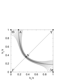
Figure 1: Notation used for special points in the Brillouin zone. The Fermi surface is shown as a black curve. Equal energy contours are shown in gray for energies between $\pm 50$meV. The dispersion used here was obtained by a 6-parameter tight binding fit to angle resolved photoemission dispersions in optimally doped Bi₂Sr₂CaCu₂O_8-δ.Eschrig00 The dispersion has a saddle point at the $M$ point. The $N$ point corresponds to the node of the $d$-wave order parameter in the superconducting state.

Extensive studies on Bi₂Sr₂CaCu₂O_8+δ as a function of temperature revealed that this characteristic shape of the spectral function is closely related to the superconducting state. In the normal state, the ARPES spectral function is broadened strongly in energy, the broadening increasing with underdoping.Ding96 The width of the spectral peak quickly decreases with decreasing temperature below $T_{c}$,Norman01 and sharp quasiparticle peaks were identified well below $T_{c}$ along the entire Fermi surface.Kaminski99 When lowering the temperature below $T_{c}$, the coherent quasiparticle peak grows at the position of the leading edge gap, and the incoherent spectral weight is redistributed to higher energy, giving rise to a dip and hump structure.Dessau91 ; Randeria95 ; Norman97 This peak-dip-hump structure is most strongly developed near the $M$-point of the Brillouin zone. The well defined quasiparticle peaks at low energies contrasts to the high energy spectra, which show a broad linewidth which grows linearly in energy.Valla99 ; Yusof01 This implies that a scattering channel present in the normal state becomes gapped in the superconducting state.Kuroda90 The high energy excitations then stay broadened, since they involve scattering events above the threshold energy. While this explains the existence of sharp quasiparticle peaks, a gap in the bosonic spectrum which mediates electron interactions leads only to a weak diplike feature.Littlewood92 This suggests that the dip feature is instead due to the interaction of electrons with a sharp (in energy) bosonic mode. The sharpness implies a strong self energy effect at an energy equal to the mode energy plus the quasiparticle peak energy, giving rise to a spectral dip.Norman98 The fact that the effects are strongest at the $M$ points implies a mode momentum close to the $(\pi,\pi)$ wavevector.Shen97

More clues are obtained by studying the dispersion of the related self energy effects. Recent advances in the momentum resolution of ARPES have led to a detailed mapping of the spectral lineshape in the high $T_{c}$ superconductor Bi₂Sr₂CaCu₂O_8+δ throughout the Brillouin zone.Bogdanov00 ; Kaminski00 The data indicated a seemingly unrelated effect near the d-wave node of the superconducting gap, where the dispersion shows a characteristic ‘kink’ feature: for binding energies less than the kink energy, the spectra exhibit sharp peaks with a weaker dispersion; beyond this, broad peaks with a stronger dispersion.Kaminski99 ; Bogdanov00 ; Kaminski00 This kink is present at a particular energy all around the Fermi surface,Bogdanov00 and away from the node, the dispersion as determined from constant energy spectra (momentum distribution curves, MDCs) shows an S-like shape in the vicinity of the kink.Norman01a The similarity between the excitation energy where the kink is observed and the dip energy at $M$, however, suggests that these effects are related.Eschrig00 Additionally, the observation that the spectral width for binding energies greater than the kink energy is much broader than that for smaller energiesKaminski99 ; Bogdanov00 ; Kaminski00 is very similar to the difference in the linewidth between the peak and the hump at the $M$ points. Further experimental studies supported the idea of a unique energy scale involved.Kaminski00 They found that away from the node, the kink in the dispersion as determined from constant momentum spectra (energy distribution curves, EDCs) develops into a ‘break’; the two resulting branches are separated by an energy gap, and overlap in momentum space. Towards $M$, the break evolves into a pronounced spectral ‘dip’ separating the almost dispersionless quasiparticle branch from the weakly dispersing high energy branch (the ‘hump’). The kink, break, and dip features all occur at roughly the same energy, independent of position in the zone,Kaminski00 the kink being at a slightly smaller energy than the break feature.Johnson01

The high energy dispersion is renormalized up to at least 200 meV and does not extrapolate to the Fermi surface crossing.Bogdanov00 ; Lanzara01 This lets us conclude that the continuum part of the bosonic spectrum coupling to the fermionic excitations extends to high energies.

Finally, there is important information contained in the doping dependence of the self energy effects. In underdoped compounds, there is a pseudogap between $T_{c}$ and $T^{\ast}$;Marshall96 ; Ding96 the pseudogap is maximal near the $M$-point of the Brillouin zone and is zero at arcs centered at the $N$-points which increase with temperature.Norman98n In the pseudogap state above $T_{c}$, there are low energy renormalizations in the dispersion, and some trace of the kink feature persists. But in the recent work by Johnson et al.Johnson01 , it was clearly shown that an additional renormalization of the dispersion sets in just at $T_{c}$. This indicates that the bosonic spectrum redistributes its spectral weight when entering the superconducting state. The additional low energy renormalization of the dispersion below the kink energy follows an order parameter like behavior as a function of temperature.Johnson01 Arguing that the renormalization near the nodal regions is influenced by the coupling to the same bosonic mode which causes the strong self energy effects at the $M$ point of the Brillouin zone, the above implies that some mode intensity may be present in the pseudogap state already, but there is an abrupt increase in the mode intensity when going from the pseudogap state into the superconducting state, and this increase shows an order parameter like behavior as a function of temperature below $T_{c}$.

The energy of the mode, as inferred from the energy separation $\Omega_{0}$ between the peak and the dip, was shown to decrease with underdoping.Campuzano99 Similarly, the kink energy is maximal at optimal doping and decreases both with underdoping and overdoping,Johnson01 indicating some relationship between the kink at the nodal $N$ point and the peak-dip-hump structure at the $M$ point. With underdoping, the sharp quasiparticle peak moves to higher binding energy, indicating that the gap increases.Campuzano99 At the same time, the spectral weight $z$ of the peak dropsCampuzano99 ; Feng00 leaving the quantity $z\Delta_{M}/k_{B}T_{c}$ roughly constant.Ding00 Also, the hump moves to higher binding energy and loses weight with underdoping.Campuzano99 This doping evolution of the quasiparticle peak points to an increasing mode intensity at the $(\pi,\pi)$ wavevector with underdoping. Again, there is a similarity to the nodal direction: the low energy renormalization of the dispersion below the kink energy increases with underdoping,Johnson01 consistent with a common origin of both effects.

II.2 C-axis tunneling spectroscopy

Unusual spectral dip features in tunneling data of Bi₂Sr₂CaCu₂O_8-δ are found in point contact junctions,Huang89 in scanning tunneling spectroscopy (STM),Renner95 ; DeWilde98 in break junctions,Mandrus91 ; DeWilde98 and in intrinsic c-axis tunnel junctions.Yurgens99 Consistently, these data show a peak feature, usually assigned to the maximal $d$-wave superconducting gap, and a hump feature at higher bias, separated from the peak by a pronounced dip feature. A characteristic of this dip feature in SIN junctions is that it occurs asymmetrically around the chemical potential, usually stronger on the occupied side of the spectrum.Huang89 ; Renner95 ; DeWilde98 This asymmetry was succesfully explained within the theoretical model presented below.Eschrig00 The dip feature has been observed in tunneling spectra of the single Cu-O₂ layer compound Tl₂Ba₂CuO₆ as well.Zasadzinski00

In order to extract information about the bosonic mode which would produce a dip feature in the tunneling conductance, a systematic study as a function of doping was performed in break junction tunneling spectroscopy by Zasadzinski et al.Zasadzinski01 There, the doping dependence in Bi₂Sr₂CaCu₂O_8-δ of the peak-dip-hump structure was determined over a wide range of doping. It was found that the dip-peak energy separation, $\Omega$, follows $T_{c}$ as $\Omega=4.9k_{B}T_{c}$. As expected for an excitonic mode, $\Omega$ approaches but never exceeds $2\Delta$ in the overdoped region, and $\Omega/\Delta$ monotonically decreases as doping decreases and the superconducting gap increases. The dip feature is found to be strongest near optimal doping. Similar shifts of the dip position with overdoping were reported prevously by STM.Renner96 Together with the ARPES results, these studies give a detailed picture about the doping dependence of the mode energy involved in electron interactions in the superconducting state.

III Coupling to the magnetic resonance mode

There have been several theoretical treatments which assigned the anomalous ARPES lineshape near the $M$ point of the zone to the coupling between spin fluctuations and electrons.Kampf90 ; Dahm96 ; Shen97 ; Norman97 ; Norman98 ; Abanov99 ; Eschrig00 The ‘collective mode model’ proposed by Norman and DingNorman98 was suggested to account for the unusual APRES lineshapes by coupling electrons to a dispersionless collective mode. The main motivation for a more detailed study of this model in Ref. Eschrig00, was to additionally account for the dispersion anomalies (‘kink’), and the isotropy and robustness of this characteristic energy scale.Kaminski00

The minimal set of characteristics for the collective mode we are interested in follows from the experimental results from ARPES and tunneling. The mode is characterized by its energy and its intensity at the $(\pi,\pi)$ wavevector (the wavevector being suggested by the momentum dependence of the strength of the ARPES anomalies). Its properties from ARPES and SIS tunneling are as follows. The energy should be weakly dependent on momentum, roughly 40 meV in optimally doped cuprates, follow $T_{c}$ with doping, and be constant with increasing temperature up to $T_{c}$. The intensity should be maximal at the $(\pi,\pi)$ wavevector, where it should increase with underdoping and follow an order parameter like behavior as a function of temperature below $T_{c}$. The mode should be absent in the normal state; a remnant can be present in the pseudogap state, but an abrupt increase in intensity should occur at $T_{c}$ with lowering temperature.

A sharp resonance with characteristics fitting the ones extracted from ARPES and tunneling measurements was observed in inelastic neutron scattering experiments on bilayer cuprates in the superconducting state, with an energy near 40 meV in optimally doped compounds.Rossat91 ; Mook93 ; Fong95 ; Bourges96 ; Fong99 A similar resonance feature at the $(\pi,\pi)$ wavevector is observed in underdoped YBa₂Cu₃O_6+x, but at a reduced energy.Dai96 ; Fong97 ; Bourges97 ; Dai99 The resonance was also found in Bi₂Sr₂CaCu₂O_8+δ, both in the optimally dopedFong99 ; He01 and overdopedHe01 regime. Recently, the resonance was discovered in single layer Tl₂Ba₂CuO₆ compound as well.He01a

To show how well the above criteria fit, we summarize its characteristics: the resonance is narrow in energy and magnetic in origin.Mook93 Its energy width is smaller than the instrumental resolution (typically less than 10 meV) for optimally and moderately underdoped materials. Strongly underdoped materials show a small broadening of the order of 10 meV.Bourges98 ; Fong00 The resonance lies below a gapped continuum, the latter having a signal typically a factor of 30 less than the maximum at $\vec{Q}$ at the mode energy.Bourges98 The mode energy decreases with underdoping, and has its maximal value of about 40 meV at optimal doping.Dai96 ; Fong97 ; Bourges97 ; Dai99 In both underdoped and overdoped regimes, the resonance energy, $\Omega_{res}$, is proportional to $T_{c}$, with $\Omega_{res}\approx 5-5.5T_{c}$.Bourges98 ; Dai99 ; Fong99 ; Fong00 ; He01

An additional aspect, specific to bilayer materials, is that it only occurs in the ‘odd’ channel, which connects the bonding combination of the bilayer bands to the antibonding one.Rossat93 The continuum is gapped in both the even and odd scattering channels (the even channel is gapped by $\approx$60 meV, even in the normal state).Reznik96 We will address this issue further below.

The resonance is strongly peaked at the $(\pi,\pi)$ wavevector. The momentum width of the spin fluctuation spectrum is minimal at the resonance energy,Bourges95 ; Bourges96 where it is (in contrast to the off-resonant momentum width) only weakly doping dependent, with a full width of about 0.22 Å^-1.Bourges95 ; Balatsky99 ; Dai01 This corresponds to a correlation length $\xi_{sfl}$ of about two lattice spacings.

A sharp resonance is not observed above $T_{c}$.Fong95 ; Bourges00 On approaching $T_{c}$ from below, the resonance energy does not shift towards lower energy,Fong95 ; Bourges96 ; Dai96 but its intensity decreases towards $T_{c}$, following an order parameter like behavior.Rossat91 ; Mook93 ; Bourges96 ; Dai96 ; Bourges00 With underdoping, the intensity at $\vec{Q}=(\pi,\pi)$ increases from about 1.6 $\mu_{B}^{2}$ for YBa₂Cu₃O₇ to about 2.6 $\mu_{B}^{2}$ per unit cell volume for YBa₂Cu₃O_6.5.Bourges98 ; Fong00 There is clearly an abrupt change in resonance intensity at $T_{c}$, even in underdoped compounds.

Note that in underdoped materials, an incommensurate response develops below the resonance energy,Dai98 which however never extends to zero energy, but instead the spectrum is limited at low energies by the so called spin gap $E_{sg}$.Dai01 This part of the spectrum behaves differently from the resonance part as a function of doping.Balatsky99 We will neglect this (weaker) incommensurate part of the spectrum in this paper.

The total spectral weight of the resonance is small and amounts to about 0.06$\mu_{B}^{2}$ per formula unit at low temperatures.Dai99 ; Fong00 We will show below that the smallness of the weight of the resonance is not an obstacle to achieving large self energy effects.

III.1 Theoretical model

We are interested in the renormalizations of the fermionic dispersion due to coupling of electrons to a sharp spin fluctuation mode at low energies, equal to about 40 meV or less. We will assume that superconducting order is already established without coupling to this resonant feature in the spin flucutation spectrum, and thus describe the superconducting state by an independent order parameter $\Delta_{k}$. This order parameter will be chosen to have $d$-wave symmetry (here and in the following the unit of length is the lattice constant $a$),

$$\Delta_{k}=\Delta_{M}(\cos k_{x}-\cos k_{y})/2$$ (1)

which takes its maximal value $\Delta_{M}$ at the $M$ point in the Brillouin zone. The magnitude $\Delta_{M}$ will be chosen so that the calculated peak in the ARPES spectrum at the $M$ point, after including self energy effects due to coupling to the spin fluctuations, fits the position of the spectral peak in experimental ARPES spectra. We stress that we do not specify the origin of the pairing interaction responsible for the order parameter $\Delta_{k}$, but the continuum part of the spin fluctuations is one of the candidates. We also underline that, as our results will show, the spin fluctuation resonance supports pairing, but does not cause superconductivity in and of itself.

In the model we employ, the retarded Green’s functions, $G^{R}_{\epsilon,k}$, for fermionic excitations in the superconducting state is a functional of the normal state electronic dispersion $\xi_{k}$, the order parameter $\Delta_{k}$, and the self energies due to coupling to spin fluctuations, $\Sigma^{R}_{\epsilon,k},\Phi^{R}_{\epsilon,k}$. The term ‘normal state’ here refers to the state at the same temperature, but with zero order parameter. We employ a six parameter tight binding fit for this dispersion, having the form

$$\xi_{k}=t_{0}+t_{1}\frac{\cos k_{x}+\cos k_{y}}{2}+t_{2}\cos k_{x}\cos k_{y}$$

$$+t_{3}\frac{\cos 2k_{x}+\cos 2k_{y}}{2}+t_{4}\frac{\cos 2k_{x}\cos k_{y}+\cos k_{x}\cos 2k_{y}}{2}$$

$$+t_{5}\cos 2k_{x}\cos 2k_{y}$$ (2)

Any set of six independent parameters for the dispersion determines the parameters $t_{0}-t_{5}$. The six parameters we use are the positions of the $N$ (node) and $A$ (antinode) points in Fig. 1, parameterized by $k_{\Gamma N}=|\vec{k}_{N}-\vec{k}_{\Gamma}|$ and $k_{MA}=|\vec{k}_{A}-\vec{k}_{M}|$, the band energies at the $M$ and $Y$ points, $\xi_{M}$ and $\xi_{Y}$, the Fermi velocity at the $N$ point, $v_{N}=|\vec{v}_{N}|$, and the inverse effective mass along direction $M-\Gamma$ at the $M$ point, $m_{M}^{-1}$. Table 1 summarizes our choices. For reference, the corresponding $t_{i}$ are (eV): $t_{0}=0.0989$, $t_{1}=-0.5908$, $t_{2}=0.0962$, $t_{3}=-0.1306$, $t_{4}=-0.0507$, and $t_{5}=0.0939$.

The parameter $\xi_{Y}$ is not known from experiment. We set it to a reasonable value to preserve a dispersion shape similar to that obtained from band theory. The inverse mass at the $M$ point is known to be negative and small in the $M-\Gamma$ direction, and it was suggested that it could be zero, giving rise to an extended van Hove singularity.Gofron94 Here we chose a finite, moderately small value. As we show, the inverse effective mass will decrease when coupling to the spin fluctuation mode is taken into account, and it is this renormalized inverse mass which is experimentally observed. Similarly, the value of the Fermi velocity at the node is chosen somewhat larger than the experimental value, since again, one observes the fully renormalized velocity; in our calculation, self energy effects renormalize this value to the moderately smaller value observed in experiment. When the doping level is varied, the band filling varies ($t_{0}$ changes), so that the van Hove singularity at the $M$ point, $\xi_{M}$, will move relative to the chemical potential. Also, the Fermi crossing $\vec{k}_{A}$ moves along the $M-Y$ line. All other band structure parameters are expected to be rather insensitive to the doping level.

Table 1: Parameters for the effective dispersion $\xi_{k}$.

$k_{\Gamma N}a$	$k_{MA}a$	$\xi_{M}$	$\xi_{Y}$	$\hbar v_{N}/a$	$\hbar^{2}/m_{M}a^{2}$
0.36$\sqrt{2}\pi$	0.18$\pi$	$-34$ meV	0.8 eV	0.6 eV	$-0.2376$ eV

The ‘normal state’ dispersion $\xi_{k}$, and the order parameter $\Delta_{k}$, are phenomenological quantities, which are already renormalized by other effects which we do not need to specify, but which are assumed to influence the physics only on an energy scale large compared to the scale of interest in this paper (50-100 meV). The self energies due to spin fluctuations will have a part due to the particle-hole continuum, and another part due to the resonance. We will consider two models, a simple form and an extended form. In the simple form, we include the effect of the continuum part of the spin fluctuation spectrum by a constant renormalization of the normal state dispersion and the order parameter. This model will capture the main physics for energies below 100 meV, which is dominated by the coupling of the electrons to the resonant spin fluctuations. The reason is the following: as we will show below, in this energy range the imaginary part of the self energies due to the continuum part of the spin fluctuations is zero, and the real part (divided by $\epsilon$) only varies weakly both in energy and momentum. This allows to approximate it by a real constant in that energy range, and thus include it into the renormalization of $\xi_{k}$ and $\Delta_{k}$. For this case, the ‘normal state’ reference is defined as the state with zero order parameter, interacting with a spin flucutation spectrum having no resonance part and a continuum part identical to that in the superconducting state. The real, physical normal state will be different because the spin fluctuation continuum changes when going from the normal to the superconducting state, leading to an additional renormalization of the dispersion. Thus, in the simple form of the model, the low energy dispersion which enters the calculations will be approximately proportional to the true normal state dispersion, but the proportionality factor will not be unity.

At higher energies, the spin fluctuation continuum can be excited, and this leads to an additional strong fermionic damping. We will study this effect in an extended model which explicitly includes the gapped spin fluctuation continuum. For this extended model, the ‘normal state’ dispersion will have a different renormalization factor as compared to the simple model above. Specifically, we use for the extended model the above dispersion scaled by the factor 1.5 and shifted back in energy, so that $\xi_{M}$ stays at its original value of $-34$meV.

We find that all essential features of the self energy effects in the superconducting state are obtained using a minimal model with a spin fluctuation spectrum shown in Fig. 2.

The continuum formally has to be cut-off at high energies. This cut-off only affects the real part of the self energy, and variation of the cut-off leads to only a weakly energy dependent contribution to the renormalization factor which can be absorbed in the dispersion $\xi_{k}$ as described above. We discuss the choice of this cut-off later.

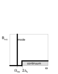
Figure 2: Left: Self energy for electrons (full lines). The wavy line denotes a spin fluctuation. Right: the model spin fluctuation spectrum we used for the wavy line in the Feynman diagram. The mode affects the low energy fermionic properties. The continuum part only couples to electrons with higher energies, and is neglected in the simple form of the model.Eschrig00 Damping of electrons at energies above 100 meV is caused by the continuum part, and is included in the extended model, which we also discuss in this paper.

The retarded Green’s function in spectral representation is given as a function of the self energies as,

$$G^{R}_{\epsilon,k}[\Sigma^{R}_{\epsilon,k},\Phi^{R}_{\epsilon,k}] = \sum_{\nu=\pm}\frac{A^{\nu}_{\epsilon,k}}{\epsilon-E^{\nu}_{\epsilon,k}+i\delta}$$ (3)

$$F^{R}_{\epsilon,k}[\Sigma^{R}_{\epsilon,k},\Phi^{R}_{\epsilon,k}] = \sum_{\nu=\pm}\frac{C^{\nu}_{\epsilon,k}}{\epsilon-E^{\nu}_{\epsilon,k}+i\delta}$$ (4)

with excitation energies $E^{\nu}_{\epsilon,k}$ and coherence factors $A^{\nu}_{\epsilon,k},C^{\nu}_{\epsilon,k}$,

$$E_{\epsilon,k}^{\pm} = \pm\sqrt{\bar{\xi}_{\epsilon,k}^{2}+|\bar{\Delta}_{\epsilon,k}|^{2}}+\delta\Sigma_{\epsilon,k}$$ (5)

$$A_{\epsilon,k}^{\pm} = \frac{1}{2}\pm\frac{\bar{\xi}_{\epsilon,k}}{2\sqrt{\bar{\xi}_{\epsilon,k}^{2}+|\bar{\Delta}_{\epsilon,k}|^{2}}}$$ (6)

$$C_{\epsilon,k}^{\pm} = \quad\pm\frac{\bar{\Delta}_{\epsilon,k}}{2\sqrt{\bar{\xi}_{\epsilon,k}^{2}+|\bar{\Delta}_{\epsilon,k}|^{2}}}$$ (7)

The renormalized dispersion and gap function are given in terms of the diagonal ($\Sigma^{R}_{\epsilon,k}$) and off-diagonal ($\Phi^{R}_{\epsilon,k}$) in particle-hole space self energies, as

$$\bar{\xi}_{\epsilon,k} = \xi_{k}+\frac{\Sigma^{R}_{\epsilon,k}+\Sigma^{R}_{-\epsilon,-k}}{2}$$ (8)

$$\bar{\Delta}_{\epsilon,k} = \Delta_{k}+\frac{\Phi^{R}_{\epsilon,k}+\Phi^{R\ast}_{-\epsilon,-k}}{2}$$ (9)

$$\delta\Sigma_{\epsilon,k} = \frac{\Sigma^{R}_{\epsilon,k}-\Sigma^{R}_{-\epsilon,-k}}{2}$$ (10)

We will couple electrons to the spin fluctuation spectrum with a coupling constant $g$, which we assume to be independent of energy and momentum. The self energies for our model are then given in terms of the spectral function of the spin fluctuations with energy $\omega$ and momentum $\vec{q}$, $B_{\omega,q}$, by the expressions (we chose a representation especially well suited for numerical studies, see App. A)

$$\Sigma^{R}_{\epsilon,k} = \sum_{\omega,q}\rho^{T}_{\omega,\epsilon-\omega}g^{2}B_{\omega,q}G^{R}_{\epsilon-\omega,k-q}$$ (11)

$$-T\sum_{\epsilon_{n},q}G^{M}_{k-q}(i\epsilon_{n})g^{2}D^{M}_{q}(\epsilon-i\epsilon_{n})$$

$$\Phi^{R}_{\epsilon,k} = \sum_{\omega,q}\rho^{T}_{\omega,\epsilon-\omega}g^{2}B_{\omega,q}F^{R}_{\epsilon-\omega,k-q}$$ (12)

$$-T\sum_{\epsilon_{n},q}F^{M}_{k-q}(i\epsilon_{n})g^{2}D^{M}_{q}(\epsilon-i\epsilon_{n})$$

where $G^{M}$ and $D^{M}$ are the fermionic and bosonic Matsubara Green’s functions which are easily expressed in terms of the spectral functions $A^{\nu}_{\epsilon,k}$ and $B_{\omega,q}$ respectively. The Matsubara sums in the second lines of Eqs. 11 and 12 only contribute to the real part of the self energies. The population factor $\rho^{T}_{\omega,\epsilon-\omega}$ is given in terms of Bose ($b$) and Fermi ($f$) population functions as,

$$\rho^{T}_{\omega,\epsilon-\omega}=b_{\omega}+f_{\omega-\epsilon}=-b_{-\omega}-f_{\epsilon-\omega}$$ (13)

We solved these equations numerically using bare Green’s functions $G^{R}_{\epsilon,k}[0,0]$, $F^{R}_{\epsilon,k}[0,0]$ for calculating the self energies $\Sigma^{R}_{\epsilon,k}$ and $\Phi^{R}_{\epsilon,k}$. We show later that feedback effects give no significant changes within our model.

Although we solve the equations above numerically without further approximations, some general remarks are in order. The function $\rho^{T}_{\omega,\epsilon-\omega}$ as a function of $\omega$ is at zero temperature nonzero only between $\omega=0$ and $\omega=\epsilon$, and is equal to sign$(\epsilon)$ in this range. Because the spin fluctuation spectrum is gapped by much more than the thermal energy in the superconducting state, we can put for all practical reasons $b_{\Omega_{res}}=0$. That means that we can neglect thermally excited modes, and only allow for emission processes at the resonant mode energy. For any gapped spin fluctuation spectrum with gap $\Omega$, the first terms in Eq. 11 and 12 are negligible in the range $-\Omega<\epsilon<\Omega$ (apart from temperature smearing near the value $\pm\Omega$). Thus, assuming that the spin fluctuation spectrum is gapped below the resonance energy, at zero temperature scattering of electronic excitations is disallowed in the interval $-\Omega_{res}<\epsilon<\Omega_{res}$. This is an expression of the fact that at least an energy $\Omega_{res}$ must be spent in order to emit one spin fluctuation mode. This is the case for optimally and overdoped cuprates. For strongly underdoped cuprates, scattering is disallowed only in the range $-E_{g}<\epsilon<E_{g}$, where $E_{g}$ is the spin gap which is smaller than $\Omega_{res}$. Also, as an implication, the renormalization function, determined by the real part of the self energy, is given in the low energy range by the second terms of Eqs. 11 and 12 only. In the following, we first consider the simple form of the model, which uses only the mode part of the spin fluctuation spectrum. After having gained some insight about the features caused by the resonance mode, we study the extended model which includes the continuum part as well.

III.2 Contribution from the spin fluctuation mode

For a sharp bosonic mode the spectral function is given by,

$$g^{2}B_{\omega,q}=2g^{2}w_{q}\left(\delta(\omega-\Omega_{res})-\delta(\omega+\Omega_{res})\right)$$ (14)

where $w_{q}$ is the energy integrated weight of the spin fluctuation mode, which is assumed to be enhanced at the $\vec{Q}=(\pi,\pi)$ point. Using the correlation length $\xi_{sfl}$, we write it as

$$w_{q}=\frac{w_{Q}}{1+4\xi_{sfl}^{2}(\cos^{2}\frac{q_{x}}{2}+\cos^{2}\frac{q_{y}}{2})}$$ (15)

We will show below that it is a good approximation to assume the mode as perfectly sharp in energy, as corrections due to the finite energy width of the mode are negligible. From neutron scattering data obtained on Bi₂Sr₂CaCu₂O_8+δ, the energy integrated weight of the resonance mode was determined as 1.9 $\mu_{B}^{2}$,Fong99 leading (after dividing out the matrix element $2\mu_{B}^{2}$) to $w_{Q}=0.95$. We fit ARPES data near optimal doping,Eschrig00 giving $g^{2}w_{Q}=0.4$eV². This implies that the coupling constant is equal to $g=0.65$ eV. This is a reliable value as discussed in Ref. Abanov01, . In Table 2, we present our minimal parameter set entering the model (we only include the parameter $\xi_{M}$ from the band structure tight binding fit, as the results are insensitive to reasonable variations of the other parameters), together with the values we used for optimally doped compounds.

Table 2: Minimal parameter set used in the calculations.

$\Delta_{M}$	$\Omega_{res}$	$\xi_{M}$	$\xi_{sfl}$	$g^{2}w_{Q}$
35 meV	39 meV	$-34$ meV	2a	0.4 eV2

III.2.1 Electron Scattering

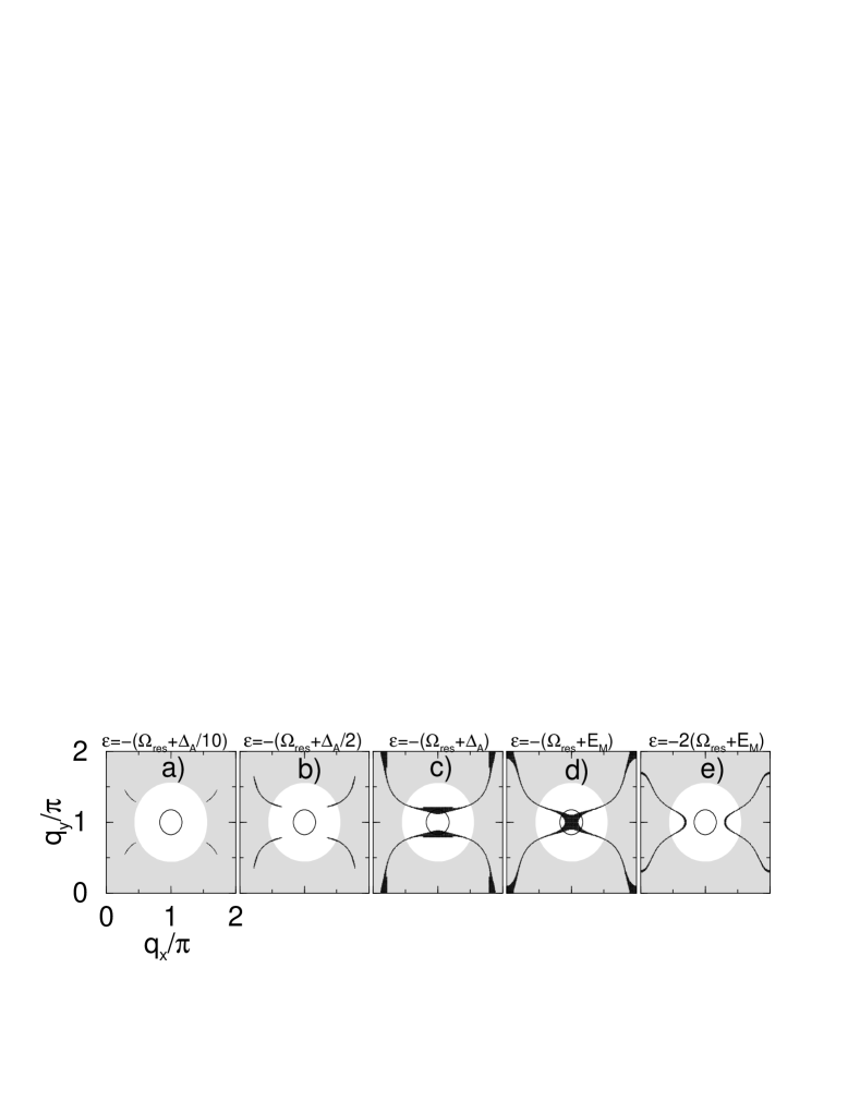
Figure 3: The black regions denote the part of the first Brillouin zone of the spin fluctuation momentum $\vec{q}$ which participates in scattering of electrons with momentum $\vec{k}_{M}$ and energy $\epsilon$, as indicated above each picture. The amount of scattering events is controlled by the form factor for the resonance mode $w_{q}$, which takes its maximal value ($w_{Q}$ ) in the center of the Brillouin zone at $\vec{Q}=(\pi,\pi)$. Inside the black circles $w_{q}>w_{Q}/2$, and inside the white region $w_{q}>w_{Q}/10$. For small energies, a), only nodal electrons are scattered. For energies equal to $\Omega_{res}+E_{M}$, d), a large region around the $M$-point of the fermionic zone participates in scattering events. Scattering electrons with this energy and momentum involves spin fluctuations with maximal weight, and thus almost exhausts the entire weight of the mode part of the spin fluctuation spectrum. Pictures c) and d) correspond to the special energies $\Omega_{res}+\Delta_{A}$ and $\Omega_{res}+E_{M}$, leading to cusp features in the energy dependence of the imaginary part of the self energy.

We first discuss phase space restrictions for electron scattering in the $d$-wave superconducting state, and how they relate to the issue of whether the small relative weight of the resonance part of the spin fluctuation spectrum leads to comparable in magnitude effects as in strong coupling superconductors. Using bare Green’s functions, the self energy at zero temperature can be written as

$$\mbox{Im}\Sigma^{R}_{\epsilon,k} = -\sum_{q}g^{2}w_{q}A^{-}_{k-q}\delta(\epsilon+\Omega_{res}+E_{k-q})$$ (16)

$$-\sum_{q}g^{2}w_{q}A^{+}_{k-q}\delta(\epsilon-\Omega_{res}-E_{k-q})$$

$$\mbox{Re}\Sigma^{R}_{\epsilon,k} = -\sum_{q}\frac{g^{2}w_{q}}{\pi}\cdot\frac{\epsilon+\left(1+\frac{\Omega_{res}}{E_{k-q}}\right)\xi_{k-q}}{(\Omega_{res}+E_{k-q})^{2}-\epsilon^{2}}$$ (17)

where $E_{k}=\sqrt{\xi_{k}^{2}+|\Delta_{k}|^{2}}$, $A^{\pm}_{k}=(1\pm\xi_{k}/E_{k})/2$. The sum over $\vec{q}$ extends over the first Brillouin zone for the spin fluctuation momentum. For negative energies, only the first sum in Eq. 16 is nonzero. The sum is a weighted average of the expression $A^{-}_{k-q}\delta(\epsilon+\Omega_{res}+E_{k-q})$ with weight factors $w_{q}$. For given fermion energies, $\epsilon$, and momenta, $\vec{k}$, the delta function restricts the allowed spin fluctuation momenta $\vec{q}$. Similar zero temperature formulas hold for the off diagonal self energy,

$$\mbox{Im}\Phi^{R}_{\epsilon,k} = -\sum_{q}g^{2}w_{q}C_{k-q}\Big{[}\delta(\epsilon-\Omega_{res}-E_{k-q})$$ (18)

$$\qquad\qquad-\delta(\epsilon+\Omega_{res}+E_{k-q})\Big{]}$$

$$\mbox{Re}\Phi^{R}_{\epsilon,k} = -\sum_{q}\frac{g^{2}w_{q}}{\pi}\cdot\frac{\left(1+\frac{\Omega_{res}}{E_{k-q}}\right)\Delta_{k-q}}{(\Omega_{res}+E_{k-q})^{2}-\epsilon^{2}}$$ (19)

with $C_{k}=\Delta_{k}/2E_{k}$.

In Fig. 3, we plot for $\vec{k}=\vec{k}_{M}$ and for several energies these restricted regions in $\vec{q}$-space. The corresponding weights for these regions, given by $w_{q}$, are maximal at $\vec{q}=\vec{Q}$ ($q_{x}=q_{y}=\pi$), and decay away from that momentum. For reference, we define the regions inside the black circle, where $w_{q}>w_{Q}/2$, and the white regions, where $w_{q}>w_{Q}/10$. The calculations were done for finite $T=40$K, and with a broadening parameter $\delta=5$ meV in Eq. 3.

For energies $-\Omega_{res}(=-39\mbox{meV})<\epsilon<0$, there is no phase space available for scattering. Scattering of electrons by the spin fluctuation mode sets in for $\epsilon=-\Omega_{res}$ at $\vec{q}$ corresponding to the wavevectors $\vec{q}=(\vec{k}_{M}-\vec{k}_{N})$ mod $(\vec{G})$, connecting the $M$ point to the nodes ($\vec{G}$ denotes a reciprocal lattice vector). In picture a) of Fig. 3, we show for $\epsilon=-(\Omega_{res}+\frac{1}{10}\Delta_{A})$ the mode wavevectors involved in scattering events. The weight for such events is very small, as can be seen from the fact that these wavevectors are outside the white region. Going further away from the chemical potential with $\epsilon$, the allowed mode wavevector regions increase, as shown in picture b) for $\epsilon=-(\Omega_{res}+\frac{1}{2}\Delta_{A})$. When the special point $\epsilon=-(\Omega_{res}+\Delta_{A})$ is reached ($=-71.2$ meV in our case), the arcs of $\vec{q}$-regions involved in scattering events close at the points $\vec{q}=(\vec{k}_{M}-\vec{k}_{A})$ mod $(\vec{G})$, as shown in picture c), and electrons are scattered strongly between the $M$ point and the $A$ points. This leads to a cusp (or peak for very small quasiparticle broadening) in the energy dependence of the imaginary part of the self energy at this energy. Going further in energy, another special point is reached at $\epsilon=-(\Omega_{res}+E_{M})$ (with $E_{M}=\sqrt{\xi_{M}^{2}+\Delta_{M}^{2}}$), at which scattering events between the $M$ points involving spin fluctuations with momentum $\vec{q}=\vec{Q}$ (and with $\vec{q}=\vec{0}$) are allowed. We show the corresponding regions in $\vec{q}$-space in picture d). This picture is important for understanding the large effect we obtain. First, the weight factor $w_{q}$ is large in the patches of phase space for allowed scattering events around $\vec{Q}$. Furthermore, because of the van Hove singularity in the band dispersion, these patches have a large area, almost filling the area inside the black circles in Fig. 3. This has as consequence that a large part of the weight of the resonance is exhausted for scattering electrons with energies equal to $\epsilon=-(\Omega_{res}+E_{M})$, which amounts to $-87.8$ meV for our parameter set. Going even further in energy, as shown in picture e), the amount of scattering events quickly decreases. The area which is involved in electron scattering events is maximal for energies between 70 meV and 90 meV. For these energies, the involved spin fluctuations are also near the $\vec{q}$-region where almost all their weight is concentrated. Thus, the strongest renormalization effects will take place in the energy range 70-90 meV.

Let us compare this discussion with the case for conventional isotropic electron-phonon coupling. In this case, the weight factors $w_{q}$ are constant. The relative amount of phonon wavevectors involved in scattering events is then equal to the ratio between the black areas shown in Fig. 3 and the total area of the Brillouin zone. This ratio is for the maximal case, picture d), equal to 5%. That means that only 5% of the total phonon weight contributes to the imaginary part of the self energy. It is well known that electron phonon coupling easily leads to renormalization factors of the order of 2. In our case, the spin fluctuation weight of the mode is only about 5% of the total spin fluctuation weight, but it is concentrated in the region inside the black circles in Fig. 3. Almost the total area inside the black circle contributes in the case of picture d), showing that the same amount of only a few percent of the bosonic spectrum is involved as well for spin fluctuations in high $T_{c}$ cuprates as for phonons in conventional strong coupling superconductors. Thus, the renormalization of the fermionic dispersion is expected to be of the same order of magnitude, and our explicit calculations confirm this.

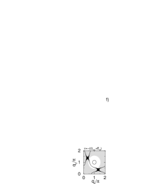
Figure 4: The same as Fig. 3 d) for a fermionic wavevector at the nodal point, $\vec{k}=\vec{k}_{N}$. Because the allowed region for scattering events is outside the region of enhanced spin fluctuations, the corresponding cusp feature in the imaginary part of the self energy is weaker than for electrons with momenta near the $M$-point.

In Fig. 4, we show the $\vec{q}$-space areas corresponding to Fig. 3 d), but for electrons near the nodal wavevector. As can be seen, the feature due to the van Hove singularity region is now weighted by a smaller value of $w_{q}$. Because of this, for nodal electrons, the corresponding peak in the self energy is smaller than for momenta near the $M$ point. It turns out that for the nodal electrons, the feature at $-(\Omega_{res}+\Delta_{A})$ is more pronounced than that at $-(\Omega_{res}+E_{M})$.

III.2.2 Renormalization factor and electron lifetime

The self energy has a characteristic shape as a function of energy, which is conserved qualitatively for all points in the Brillouin zone. This is a consequence of the fact that all points are coupled via the spin fluctuation mode, which has a finite width in momentum, to all special points in the Brillouin zone with their corresponding characteristic energies. These special points are the nodal $N$ points, and the van Hove singularities at the $M$ points and the $A$ points (the latter is a dispersion maximum in the superconducting state). Because the general shape of the energy dependence of the self energy does not vary much with momentum (although the overall intensity does), it is sufficient to discuss the important features in the energy dependence of the self energy at the $M$ point.

We numerically evaluated the self energy, using a broadening parameter $\delta=5$ meV. In Fig. 5, we show the results for the renormalization function and electron scattering rate at the $M$ point,

$$Z_{M}(\epsilon)=1-\frac{\mbox{Re}\,\delta\Sigma_{M}(\epsilon)}{\epsilon}\qquad\Gamma_{M}(\epsilon)=-\mbox{Im}\,\delta\Sigma_{M}(\epsilon)$$ (20)

as a function of energy.

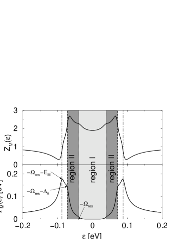
Figure 5: Renormalization factor at the $M$ point, $Z_{M}(\epsilon)$ (top) and electron scattering rate at the $M$ point, $\Gamma_{M}(\epsilon)$ (bottom). The thin lines denote some characteristic energies: $\pm\Omega_{res}$ (dotted), $\pm(\Omega_{res}+\Delta_{A})$ (dashed), and $\pm(\Omega_{res}+E_{M})$ (dot-dashed). Electrons at low temperatures are scattered only if their energy is larger than $\Omega_{res}$, so that they are able to emit a collective mode excitation. The parameters used are: $T=40$K, $\Omega_{res}=$39 meV, $\Delta_{M}=$35 meV.

There are three characteristic energies (in addition to temperature, which smears all features by $k_{B}T$). Region I is bounded by the resonance energy, $\Omega_{res}$, and has zero scattering rate at zero temperature (this statement is true for electrons at any point in the Brillouin zone). At finite temperature, a region $k_{B}T$ around $\pm\Omega_{res}$ allows for a small amount of scattering, even in region I. Because states are occupied near the $M$ point, we will only discuss negative energies in the following. At $\epsilon=-\Omega_{res}$, scattering for all electrons in the Brillouin zone sets in due to coupling to nodal electrons via emission of a spin fluctuation mode. Absorption processes are negligible due to the large (compared to temperature) mode energy. In region II, a larger and larger area around the nodes participates in scattering events, (as can be seen from pictures a and b in Fig. 3), until finally the point at the zone boundary with maximal gap, $\pm\Delta_{A}$, is reached (picture c in Fig. 3). This point corresponds in Fig. 5 to a cusp feature in the imaginary part of the self energy at $-(\Omega_{res}+\Delta_{A})$. The third feature, at $-(\Omega_{res}+E_{M})$, corresponds to the van Hove singularity at the $M$ point of the Brillouin zone, which is close to the chemical potential in cuprates (picture d in Fig. 3). The proximity of this van Hove singularity leads to a stronger peaked feature in the scattering rate near $\pm(\Omega_{res}+\Delta_{A})$ compared to the case where this van Hove singularity at the $M$ point is absent. The renormalization factor is rather constant in region I as a consequence of its connection to the imaginary part via Kramers-Kronig relations. The enhancement in regions I and II compared to unity comes from two step features at $\pm(\Omega_{res}+E_{M})$ and at $\pm(\Omega_{res}+\Delta_{A})$. Note that the step feature due to the van Hove singularity at the $M$ point contributes about 50% to the total enhancement. The small features at $\pm\Omega_{res}$ are due to the finite lifetime of the electrons involved in scattering processes as discussed below. The onset of scattering at the emission edge for the spin fluctuation mode occurs as a jump if the electrons involved have a finite spectral width. At even higher energies, corresponding to Fig. 3 e), the scattering due to the spin fluctuation mode becomes less effective. Note that the spectral peak of the electrons at $\pm\Delta_{k}$ is either in region I or in region II. Thus, quasiparticles near the nodal regions are always sharper in energy then quasiparticles near the maximal gap regions. In overdoped cuprates, the maximal gap is usually smaller than the mode energy, so that for the broadening of the quasiparticle peaks, the spin fluctuation mode is not relevant.

For the following discussion, it is useful to derive approximate analytical expressions. At zero temperature, using Eq. 17, we obtain

$$Z_{M}(\epsilon)=1+\sum_{q}\frac{g^{2}w_{q}}{\pi}\frac{1}{(\Omega_{res}+E_{k_{M}-q})^{2}-\epsilon^{2}}$$ (21)

The main contribution comes from the regions where $E_{k_{M}-q}$ is less than 100 meV. We can estimate those regions by the requirement that $\vec{k}_{M}-\vec{q}$ is in the area around the $M$ points deliminated by $\pm 0.35\pi$ in $M-Y$ direction and by about 0.3$\pi$ along the $M-\Gamma$ direction. Then, replacing $\Delta_{k_{M}-q}$ by $-\Delta_{M}$, and $E_{k_{M}-q}$ by $E_{M}$, we perform the $\vec{q}$-sum over that area of the function $w_{q}$. We denote $\sum_{q}w_{q}$ over this area by $I_{0}$. For our model we have $I_{0}=0.035$. Using this approximation, we obtain

$$Z_{M}(\epsilon)\approx 1+\frac{g^{2}I_{0}}{\pi}\frac{1}{(\Omega_{res}+E_{M})^{2}-\epsilon^{2}}+\lambda_{M}^{(N)}(\epsilon)$$ (22)

Here, $\lambda_{M}^{(N)}(\epsilon)$ denotes the contributions coming from the regions where $\vec{k}^{\prime}=\vec{k}_{M}-\vec{q}$ is outside of the above range. It is dominated by contributions where $\vec{k}^{\prime}$ is near the nodal regions of the Brillouin zone, thus the relevant spin fluctuation momentum is $\vec{q}=(\vec{k}_{M}-\vec{k}_{N})$ mod $\vec{G}$. The contribution $\lambda_{M}^{(N)}$ is smaller than the first term in Eq. 22, but not negligible. Because Eq. 22 neglects the dispersion between $(\Omega_{res}+\Delta_{A})$ and $(\Omega_{res}+E_{M})$ near the $M$ point, it should be used for energies not too close to the region between these two values. We will make use of this formula below for energies near $\epsilon=E_{M}$, where this formula gives a good approximation.

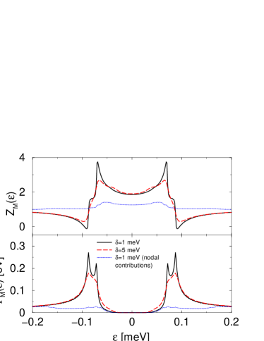
Figure 6: Renormalization factor at the $M$ point, $Z_{M}(\epsilon)$ (top) and electron scattering rate at the $M$ point, $\Gamma_{M}(\epsilon)$ (bottom). The picture compares results for two different residual quasiparticle linewidths: $\delta=1$ meV (full lines) and $\delta=5$ meV (dashed lines). As dotted lines the nodal contributions, when restricting the quasiparticle momenta to the regions outside the area around the $M$ points discussed in the text, is shown for $\delta=1$ meV.

III.2.3 The quasiparticle scattering rate

For overdoped materials the quasiparticle peak at the $M$ point is situated below the onset of scattering due to emission of spin fluctuations. In this case the width is determined by other processes, and we model this residual quasiparticle width by a parameter $\delta$. In Fig. 6, we show the influence on the renormalization factor and the scattering function of the residual quasiparticle width. We compare the results for $\delta=5$ meV with those for $\delta=1$ meV. For very small quasiparticle broadening (full lines) the cusp features in the imaginary part of the self energy turn into peaks (which ultimately evolve into square root singularities for perfectly sharp quasiparticles and resonance). The second feature to mention is that the scattering rate near the onset points, $\pm\Omega_{res}$, is influenced strongly by the residual quasiparticle width. Because this onset region governs the quasiparticle width in underdoped cuprates, as we show later, we study it in the following in more detail. In the lower part of Fig. 6 we show as a dotted line the contribution to the electron scattering rate coming from the final states not too close to the $M$ points (the regions which determine $\lambda_{M}^{(N)}$, introduced above) as compared to the full scattering rate (full line). It is clearly seen that the sharp features come from the $M$ point regions, whereas the nodal regions contribute to the onset of electron scattering and provide a smooth constant background at higher energies.

The behavior of the imaginary part of the self energy near the onset points, $\pm\Omega_{res}$, in Figs. 5 and  6 is determined by the nodal electrons. For larger residual quasiparticle widths ($\delta=5$ meV, dashed lines in Fig.  6) there are states available at the chemical potential (coming e.g. from impurity scattering), which increase the number of final states for scattering events. Thus, the onset in Fig.  6 for the electron scattering rate is stronger in this case than for $\delta=1$ meV. For zero temperature there will be a jump at energy $\pm\Omega_{res}$ in the imaginary part of the self energy, which causes the small cusps at the same energy in the renormalization factor (top panel in Fig. 6). For $\delta=0$ the onset is linear in energy.

We will estimate analytically the onset behavior near these points for the case $\delta=0$ now. For this we use Eqs. 10 and  16. We replace $\vec{q}$ by $\vec{k}^{\prime}-\vec{k}$, approximate $w_{q}$ by $w_{MN}=w_{k_{M}-k_{N}}$, and linearize the dispersion around the nodes, $\Delta_{k}=\vec{v}_{\Delta}(\vec{k}^{\prime}-\vec{k}_{N})$, $\xi_{k}=\vec{v}_{N}(\vec{k}^{\prime}-\vec{k}_{N})$. Here $\vec{v}_{\Delta}=\partial_{k}\Delta_{k}$ and $\vec{v}_{N}=\partial_{k}\xi_{k}$ taken at the $N$ point. For our model, we have $v_{\Delta}=\Delta_{M}\sin(k_{xN})/\sqrt{2}$, which is valid near optimal doping. (But note that for underdoped cuprates, $v_{\Delta}$ was experimentally shown to be smaller than that value, perhaps scaling with $k_{B}T_{c}$ instead of with $\Delta_{M}$.Mesot99 ) Performing the $\vec{k}^{\prime}$ sum and summing over all four nodes, we arrive at

$$\mbox{Im}\delta\Sigma_{M}^{(N)}(\epsilon) = -\frac{g^{2}w_{MN}}{\pi v_{N}v_{\Delta}}(|\epsilon+\Omega_{res}|\Theta(-\epsilon-\Omega_{res})$$ (23)

$$\qquad+|\epsilon-\Omega_{res}|\Theta(\epsilon-\Omega_{res}))$$

Here, the $\Theta$-function is unity for positive argument and zero otherwise. Thus, the slope of the scattering rate at $\epsilon=\pm\Omega_{res}$ is given by $\mp g^{2}w_{MN}/\pi v_{N}v_{\Delta}$. For the parameters in Tables 1 and 2, the magnitude of this slope is equal to 9.5 $w_{MN}/w_{Q}\approx 0.56$. Note that Eq. 23 gives a good approximation of the scattering rate in the interval $\Omega_{res}<|\epsilon|<\Omega_{res}+\Delta_{A}/2$. For energies further away from the onset, the change of the quantity $v_{\Delta}$ (which goes to zero at the $A$ point) leads to a stronger increase. Finally, for underdoped cuprates the excitation energy at the $M$ point, $E_{M}$, is larger than $\Omega_{res}$. Then, the quasiparticle linewidth at the $M$ point is given by $-\mbox{Im}\delta\Sigma_{M}^{(N)}(-E_{M})/Z_{M}(-E_{M})$. Thus, for underdoped cuprates it is given by,

$$\tilde{\Gamma}_{M} = \frac{g^{2}w_{MN}}{\pi v_{N}v_{\Delta}}\frac{E_{M}-\Omega_{res}}{Z_{M}}$$ (24)

with $Z_{M}\equiv Z_{M}(-E_{M})$. Near the nodes, on the contrary, the quasiparticles will stay relatively sharp even in underdoped compounds because the peaks positions are then below the onset energy $\pm\Omega_{res}$.

III.2.4 The coupling constant and the weight of the spin resonance

One potential criticism of a model which assigns the observed anomalies in the dispersion to coupling of electrons to the spin resonance mode is the spectral weight of the resonance, $I_{0}$, which amounts to only a few percent of the local moment sum rule.Kee01 Our calculations show that this is not an obstacle,Abanov01 as we obtain a dimensionless coupling constant of order one, as observed experimentally.

Here we estimate $\lambda_{M}$, given by $Z_{M}(0)-1$, for the resonance mode. From Eq. 22, it is equal to

$$\lambda_{M} \approx \frac{g^{2}I_{0}}{\pi}\cdot\frac{1}{(\Omega_{res}+E_{M})^{2}}+\lambda_{M}^{(N)}(0)$$ (25)

Using values for optimal doping (Table 2), the first term in this sum is equal to $17.44I_{0}$, which amounts to about 0.61 (in our model $I_{0}=0.035$). This is already a large part of the total coupling constant, which from Fig. 5 is $\lambda_{M}\approx 0.9$. The contribution $1+\lambda_{M}^{(N)}(\epsilon)$ is shown as dotted line in the upper part of Fig. 6. $\lambda_{M}^{(N)}$ is not negligible, but contributes about 30% to the total coupling constant.

We obtain an analytic formula for the low energy correction to the renormalization factor due to scattering between nodal points and $M$ points, $\lambda_{M}^{(N)}(\epsilon)$, by a Kramers-Kronig transform of $\mbox{Im}\Sigma_{M}^{(N)}(\epsilon)$, in which only energies up to a cut-off $\pm(\Omega_{res}+\Delta_{A})$ are taken into account, and replacing $\mbox{Im}\Sigma_{M}^{(N)}(\epsilon)$ above this cut-off by a constant (see the dotted lines in Fig. 6) equal to its value at the cut-off. The result for $\epsilon=0$ is,

$$\lambda_{M}^{(N)}(0)\approx\frac{g^{2}w_{MN}}{\pi v_{N}v_{\Delta}}\frac{2}{\pi}\ln\left(1+\frac{\Delta_{A}}{\Omega_{res}}\right)$$ (26)

For our parameter set this amounts to $\lambda_{M}^{(N)}(0)\approx 0.21$. Note that $\lambda_{M}^{(N)}$ increases with decreasing $\Omega_{res}$.

To summarize, dimensionless coupling constants (comparable to those for strong-coupling electron-phonon systems) are easily achieved with reasonable parameters by coupling electrons to the spin resonance.

III.2.5 Particle hole asymmetric renormalizations

From Eq. 17, we see that the second term in the numerator, proportional to $\xi_{k-q}$, affects the band dispersion $\xi_{k}$. The resulting renormalization is given by,

$$\bar{\xi}_{\epsilon,k}=\xi_{k}-\sum_{q}\frac{g^{2}w_{q}}{\pi}\cdot\frac{\left(1+\frac{\Omega_{res}}{E_{k-q}}\right)\xi_{k-q}}{(\Omega_{res}+E_{k-q})^{2}-\epsilon^{2}}$$ (27)

From this formula, it is clear that notable renormalizations of the Fermi surface only take place if $\xi_{k-q}$ is not too far from (but also not at) the chemical potential. Thus, the largest renormalizations are expected at the $M$ point regions of the Brillouin zone.

In Fig. 7 (left), we show the particle-hole asymmetric part of the self energy as a function of $\epsilon$ for electrons at the $M$ point of the Brillouin zone. The imaginary part shows a peak due to the van Hove singularity at the $M$ point, but the cusp feature due to the $A$ points is missing, because points where $\vec{k}-\vec{q}$ is on the Fermi surface do not contribute to the sum in Eq. 27. The real part indicates that the renormalization of the dispersion is confined to energies between $-\Omega_{res}-E_{M}$ and $\Omega_{res}+E_{M}$. Using the same approximation procedure as above, we obtain for the renormalization at the $M$ point,

$$\bar{\xi}_{M}(\epsilon)\approx\xi_{M}\left(1-\frac{g^{2}I_{0}}{\pi}\frac{1}{E_{M}}\frac{\Omega_{res}+E_{M}}{(\Omega_{res}+E_{M})^{2}-\epsilon^{2}}\right)$$ (28)

The first important point is that the renormalization has opposite sign to $\xi_{k}$, thus the band is renormalized towards the chemical potential. In particular, there is a ‘pinning’ effect of the van Hove singularity at the $M$ point to the chemical potential, as long as $\xi_{M}$ is of the order of $\Omega_{res}$. Furthermore, the renormalization factor $Z_{M}(\epsilon)$ from Eq. 22 increases this effect, as $\bar{\xi}_{M}/Z_{M}$ defines the quasiparticle dispersion.

Figure 7: Left: The part of the self energy (eV) defining the band renormalization at the $M$ point as a function of energy, for $\Delta_{M}$=35 meV, $\Omega_{res}$=39 meV, and $g$=0.65 eV. Right: The quantity $\bar{\xi}_{M}(\epsilon)/(Z_{M}(\epsilon)\xi_{M})$ (filled circles) and $1/Z_{M}(\epsilon)$ (empty circles) for $\epsilon=-\Delta_{M}$ as a function of the coupling constant $g$.

In order to quantify this, we show in the right panel of Fig. 7 the relative changes of the dispersion, $\bar{\xi}_{M}(\epsilon)/(Z_{M}(\epsilon)\xi_{M})$ (filled circles), in comparison to the inverse renormalization factor $1/Z_{M}(\epsilon)$ (empty circles). The latter would give the band renormalization in the absence of particle hole asymmetric parts in the self energy. As can be seen in this figure, the band is renormalized towards the chemical potential and even crosses it for large coupling constants. For coupling constants near 0.6 eV, the renormalized band is close to the chemical potential. Thus, the dispersion of the peak in ARPES is negligible in the $M$ point regions as a result of the renormalization of the dispersion. The renormalization of the band implies an increase in the chemical potential, so as to keep the particle density constant. This effect would increase the distance between the chemical potential and the van Hove singularity at the $M$ point, leading to an equilibrium value in a self consistency loop. We did not solve this self consistency problem, but assumed that our parameter choice is close enough to the self consistent solution to capture the main physics.

III.2.6 Off diagonal self energy

In order to understand the renormalization of the order parameter $\Delta_{k}$ due to coupling to the resonance mode, we observe from Eq. 19,

$$\bar{\Delta}_{\epsilon,k}=\Delta_{k}-\sum_{q}\frac{g^{2}w_{q}}{\pi}\frac{\left(1+\frac{\Omega_{res}}{E_{k-q}}\right)\Delta_{k-q}}{(\Omega_{res}+E_{k-q})^{2}-\epsilon^{2}}$$ (29)

This formula is very similar to that for the band renormalization, except that the order parameter at momentum $\vec{k}-\vec{q}$ now determines the renormalization effect. Note that if $w_{q}$ were independent of $\vec{q}$, no renormalization would take place due to the $d$-wave symmetry of the order parameter. Since the spin fluctuation continuum, which we discuss later, is very broad in momentum, the renormalization effects in the off-diagonal components is dominated by the resonance contribution. As the order parameter vanishes at the node, we concentrate on the renormalization near the $M$ point region again. Adopting the approximations as above (note that contributions from the nodal regions cancel because of the $d$-wave symmetry), and using Eq. 19, we arrive at

$$\frac{\bar{\Delta}_{M}(\epsilon)}{\Delta_{M}}\approx 1+\frac{g^{2}I_{0}}{\pi}\frac{1}{E_{M}}\frac{\Omega_{res}+E_{M}}{(\Omega_{res}+E_{M})^{2}-\epsilon^{2}}$$ (30)

The positive sign is due to the fact that $\Delta_{M+Q}=-\Delta_{M}$. As a result of this, there will be a compensating effect when calculating the quantity $\bar{\Delta}_{M}(\epsilon)/Z_{M}(\epsilon)$, which determines the peak position. In Fig. 8 (left), the real and imaginary parts of the off diagonal self energy at the $M$ point are shown. The imaginary part is relevant only for energies with absolute value $>\Omega_{res}+\Delta_{A}$. For smaller energies, the main effect is to increase the magnitude of the order parameter $\Delta_{k}$ in the energy range $-\Omega_{res}-\Delta_{A}<\epsilon<\Omega_{res}+\Delta_{A}$. Note that the self energy due to coupling to the resonance mode has $d$-wave symmetry, like the order parameter. Thus, the coupling to the resonance mode supports superconductivity. In order to quantify the amount that the resonance mode contributes to the spectral gap, we show in Figs. 8 (right) and 9 the quantity $\bar{\Delta}_{M}(\epsilon)/(Z_{M}(\epsilon)\Delta_{M})$ (together with $1/Z_{M}(\epsilon)$ for comparison) as a function of three different parameters: $g$, $\Delta_{M}$, and $\Omega_{res}$.

As can be seen from these figures, although the renormalization factor $Z_{M}$ would reduce the order parameter considerably, the off diagonal contribution to the self energy from coupling of electrons to the resonance mode restores the gap to its original value. Thus, the resonance contribution to the gap is as big as that from other sources, and starts to dominate if the coupling constant exceeds about 0.5 eV.

Figure 8: Left: The off diagonal self energy (eV) at the $M$ point of the Brillouin zone as a function of $\epsilon$ is shown for coupling constant $g$=0.65 eV. Right: The quantities $\bar{\Delta}_{M}(\epsilon)/(Z_{M}(\epsilon)\Delta_{M})$ (filled circles) and $1/Z_{M}(\epsilon)$ (empty circles) are shown for $\epsilon=-\Delta_{M}$ as a function of the coupling constant $g$. Parameters used are $\Delta_{M}$=35 meV, $\Omega_{res}$=39 meV.

Figure 9: The quantities $\bar{\Delta}_{M}(\epsilon)/(Z_{M}(\epsilon)\Delta_{M})$ (filled circles) and $1/Z_{M}(\epsilon)$ (empty circles) are shown for $\epsilon=-\Delta_{M}$ as a function of $\Delta_{M}$ (left, for $g=0.65$ eV and $\Omega_{res}=39$ meV) and $\Omega_{res}$ (right, for $g=0.65$ eV and $\Delta_{M}=35$ meV).

The reason why $\bar{\Delta}_{M}(\Delta_{M})$ is so close to $Z_{M}(\Delta_{M})\Delta_{M}$ is that the additional factor $1+\Omega_{res}/E_{M}$ in Eq. 30 compared to Eq. 22 is approximately canceled by the presence of the additional $\lambda_{M}^{(N)}(\Delta_{M})$ in Eq. 22. An analogous term in Eq. 30 is missing due to the sign change of the order parameter at the node. The degree to which this cancellation holds is a surprising numerical result and allows us to avoid a self consistency loop for the determination of $\Delta_{M}$ near optimal doping. Thus, the experimental parameters which enter our calculations are already sufficiently self consistent.

III.2.7 Spectral functions at the $M$ point

In this part, we discuss the spectral lineshape, which is an experimentally accessible quantity. The main features of the spectral lineshape are captured in the simple model neglecting the continuum part of the bosonic spectrum. We discuss in the following the influence of the different parameters of the theory on the spectral function,

$$A(\epsilon,\vec{k}_{M})=-2\mbox{Im}G^{R}(\epsilon,\vec{k}_{M})$$ (31)

and will discuss changes due to the continuum part of the spin fluctuation spectrum later. In our numerical studies, we used a broadening parameter $\delta=5$ meV. This accounts for processes not covered by scattering by spin fluctuations.

In Fig. 10, we present the results for the spectral function at the $M$ point of the Brillouin zone for both a perfectly sharp resonance and for a finite width of the resonance of 10 meV. It is obvious that the energy width of the resonance has very little effect on the ARPES spectra, except a slight reduction of the peak height.

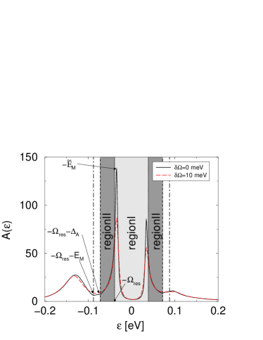
Figure 10: Spectral functions at $M$ for a perfectly sharp resonance (full line) and for a resonance with a finite energy width of 10 meV (dashed line). Parameters are for optimal doping. The finite width of the mode has very little influence on the ARPES spectra, and can be neglected for most purposes.

Thus, we will concentrate all our following discussions on a perfectly sharp resonance mode. The main features of the spectral function is the dip feature at an energy of about the resonance energy relative to the peak. The peak position at $-\tilde{E}_{M}$ is renormalized by self energy effects discussed above, and is shifted from the bare $-E_{M}$ to be near $-\Delta_{M}$. The dip feature is actually spread out over a range of size $E_{M}-\Delta_{A}$, and it is the onset of this dip feature which defines the resonance energy, $\Omega_{res}$. The dip feature is followed by a hump at higher binding energies, and the position of the hump maximum is very sensitive to the coupling constant and to damping due to the spin fluctuation continuum, as we show later. Thus, we concentrate in the following on the peak-dip structure. Another feature worth mentioning is the asymmetry of the lineshape at positive and negative binding energies, with a relatively weak dip feature on the unoccupied side compared to the occupied side.

In Fig. 11 (left), the effect of a varying resonance energy $\Omega_{res}$ (keeping all other parameters at their values for optimal doping) is shown. The spectral function shows two effects. First, the peak weight is reduced with decreasing mode energy. Second, as soon as the quasiparticle excitation energy exceeds $\Omega_{res}$, strong damping sets in. We can understand these results in the light of the discussion for the self energy. As we mentioned above, the scattering rate has a gap equal to $\Omega_{res}$. Thus, as long as the spectral peak is situated below that energy, in region I of Figs. 10 and 5, there will be no damping, and the peak width is set by the residual broadening due to other processes. If the peak is positioned above $\Omega_{res}$ (region II in Fig. 10), it feels the self energy in region II of Fig. 5, and will be broadened. Because in region II the self energy is dominated by scattering processes involving nodal electrons, the width in this region is set by the imaginary part of the self energy divided by the renormalization factor, and is given in Eq. 24. At the same time, for decreasing resonance mode energy, the incoherent part of the spectral function grows, taking weight from the quasiparticle peak.

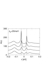
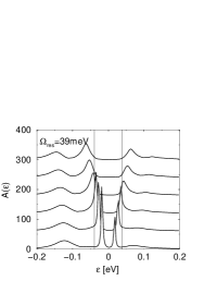
Figure 11: Spectral functions at the $M$ point for varying $\Omega_{res}$ (left, for 10 meV, 20 meV, 30 meV and 40 meV from bottom to top; the thin lines denote the value $\pm\Delta_{M}$), and for varying $\Delta_{M}$ (right, for 15 meV, 25 meV, 35 meV, 45 meV, 55 meV, and 65 meV from bottom to top; the thin lines denote the value $\pm\Omega_{res}$). All other parameters are kept fixed at their optimal doping values. The spectra are offset for clarity.

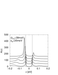
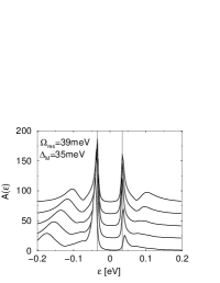
Figure 12: Spectral functions at the $M$ point for varying coupling constant (left, $g=$ 0.1 eV, 0.3 eV, 0.5 eV, 0.7 eV, and 0.9 eV from top to bottom; thin lines denote $\pm\Delta_{M}$) and for varying distance of the van Hove singularity at the $M$ point from the chemical potential (right, for $-\xi_{M}=$ 0 meV, 20 meV, 40 meV, 60 meV, and 100 meV from top to bottom; thin lines denote $\pm\Delta_{M}$). All other parameters are kept fixed at their optimal doping values. The spectra are offset for clarity.

Thus, in Fig. 11, which is for $\Delta_{M}=$35 meV, the quasiparticle weight increases from the lowest curve (for $\Omega_{res}=$ 10 meV) to the uppermost curve (for $\Omega_{res}=$ 40 meV). Simultaneously the broadening decreases. As the onset of quasiparticle damping and the loss of the coherent part of the spectrum is a result of a decreasing resonance mode energy relative to the gap, the same effect is expected by increasing the gap keeping the resonance mode energy constant. This is shown in Fig. 11 (right). In this case, the onset of quasiparticle damping is always at the same energy $\Omega_{res}=$39 meV, but for the lowest curve, corresponding to a small gap of 15 meV, quasiparticle peaks are well established, whereas for the uppermost curve, corresponding to a large gap of 65 meV, the quasiparticle peaks are strongly broadened. However, in this case, the weight of the peak is affected only weakly, as we will discuss below.

Finally, we show in Fig. 12 the influence of increasing coupling $g$, and of an increasing distance of the van Hove singularity from the chemical potential, $\xi_{M}$. In both cases, the hump energy is strongly affected, moving to higher binding energy with increasing coupling and increasing $\xi_{M}$. In the left panel, one can also see that the weight of the peak is strongly reduced with increasing coupling constant. This is not the case with varying $\xi_{M}$, as seen from the right panel in Fig. 12, and will be discussed in more detail below.

III.2.8 The coherent quasiparticle weight of the ARPES spectrum

Although one can define a quasiparticle residue via the renormalization factor $Z(\epsilon)$, in light of the experimental studies, we will in this part study the weight of the quasiparticle peak in the ARPES spectrum, determined by numerically integrating over the peak region. For strongly renormalized spectra, this experimentally motivated quantity will differ from the first. We note that due to coupling to the mode, the peak weight is reduced and redistributed to the hump. Because the peak weight in the experimental literature is often referred to as the ‘coherent quasiparticle weight’, we will use the same terminology here.

We consider the spectral function at the $M$ point of the Brillouin zone. Because the peak is separated from the hump by a dip which extends from $-\epsilon_{1}=-(\Omega_{res}+\Delta_{A})$ to $-\epsilon_{2}=-(\Omega_{res}+E_{M})$, we define as the coherent quasiparticle weight the quantity,

$$z_{M}=-\frac{1}{\pi}\int_{-\epsilon_{1}}^{0}\;d\epsilon\;\mbox{Im}G^{R}_{M}(\epsilon)$$ (32)

Without interactions between the quasiparticles, $z=0.5$ at the Fermi surface, because the quasiparticle peaks at $\pm\Delta$ in BCS theory each have one half of the total weight; the value at negative energy is somewhat larger than 0.5 at the $M$ point because it is an occupied state. Coupling of the quasiparticles to the mode reduces $z$. In Figs. 13 and 14, our numerical studies are summarized. The results are as follows: (1) $z_{M}$ is only weakly dependent on the gap and the band structure in the relevant parameter range; (2) $z_{M}$ is proportional to the mode energy $\Omega_{res}$; together with the experimental finding $\Omega_{res}\propto k_{B}T_{c}$, this means $z_{M}\propto k_{B}T_{c}$; (3) for coupling constants of order the band width or larger, $z_{M}\propto 1/(g^{2}w_{Q})$; for smaller coupling constants, $1/z_{M}\sim A+Bg^{2}w_{Q}$ with $A$ and $B$ constants; (4) $z_{M}$ weakly decreases with increasing antiferromagnetic correlation length $\xi_{sfl}$. We can understand some of these features using the approximate expression of Eq. 22. Evaluating $Z_{M}(\epsilon)$ at $\epsilon=-E_{M}$, and taking into account the coherence factor at the $M$ point, $A^{-}_{M}\equiv A^{-}_{M}(-E_{M})$, and the nodal renormalization factor $Z_{M}^{(N)}\equiv 1+\lambda_{M}^{(N)}(-E_{M})$, gives

$$z_{M} \approx \frac{\Omega_{res}A^{-}_{M}}{Z_{M}^{(N)}\Omega_{res}+\frac{g^{2}I_{0}}{\pi(\Omega_{res}+2E_{M})}}$$ (33)

which defines the constants $A$ and $B$.

Figure 13: The coherent quasiparticle weight as a function of $\Delta_{M}$ (left) and $\xi_{M}$ (right) for $\Omega_{res}=$39 meV. Although the peak width changes considerably as a function of $\Delta_{M}$, the peak weight is only weakly dependent on $\Delta_{M}$ and $\xi_{M}$.

Figure 14: The inverse of the coherent quasiparticle weight $1/z$ is approximately a linear function of $g^{2}w_{Q}$ (left). Here we have chosen $\Omega_{res}=$39 meV and $\Delta_{M}=$35 meV. The right panel shows that $z$ is proportional to $\Omega_{res}$.

In the underdoped region, where $\Omega_{res}$ is much smaller than $2E_{M}$, we can approximate further to obtain

$$z_{M} \approx \frac{2\pi E_{M}\Omega_{res}A^{-}_{M}}{g^{2}I_{0}}$$ (34)

Here, we neglected the first term in the denominator of Eq. 33 compared to the second, which is justified when $z_{M}$ is small. In the overdoped region, where $g^{2}I_{0}$ decreases and $\Omega_{res}$ approaches $2\Delta_{h}$ (where $\Delta_{h}$ is the gap at the hot spots), this scaling with $\Omega_{res}$ should break down according to Eq. 33. Note that experimentally, the relation $\Omega_{res}\approx 4.9k_{B}T_{c}$ was shown,Zasadzinski01 and also the relation

$$\left(\frac{z_{M}E_{M}}{k_{B}T_{c}}\right)_{(exp)}\approx 0.5$$ (35)

was experimentally found.Ding00 Thus, our expression Eq. 34 would be consistent with the experimental finding if with doping $E_{M}^{2}$ scaled with $g^{2}I_{0}$. Within our theory this experimental finding can be interpreted as an indication that the phenomenological order parameter $\Delta_{k}$ is governed by the same coupling constant $g$.

III.3 Contribution of the spin fluctuation continuum

At energies higher than that corresponding to the continuum edge of the spin fluctuation spectrum, additional broadening due to coupling to that part of the spectrum sets in. Because the continuum extends to electronic energies ($\sim$ eV), the introduced scattering rate will increase continuously with energy up to electronic energies as well. We model the continuum part by

$$g^{2}B^{c}_{\omega,q}=2g^{2}c_{q}\left(\Theta(\omega-2\Delta_{h})-\Theta(-\omega-2\Delta_{h})\right)$$ (36)

where the gap in the continuum spectrum is given by $2\Delta_{h}$. This form for the gapped continuum is similar to the gapped marginal Fermi liquid spectrum considered earlier by other authors. Littlewood92 ; Norman98 The momentum dependence takes into account the experimentally observed flatter behavior around the $(\pi,\pi)$ wavevector at higher energies, and is modeled as

$$c_{q}=c_{Q}\left(\frac{1+(32\xi_{c}^{4})^{-1}}{1+16\xi_{c}^{4}(\cos^{4}\frac{q_{x}}{2}+\cos^{4}\frac{q_{y}}{2})}-(32\xi_{c}^{4})^{-1}\right)$$ (37)

with a correlation length $\xi_{c}=0.5a$ compatible with experimental findings. We subtracted a background term, so that the response far away from the $(\pi,\pi)$ wavevector is small, as experimentally observed (we have chosen this background term so that $c_{q}$ is zero at $\vec{q}=0$).

For the chosen correlation length, the momentum average of $c_{q}$ gives $0.5c_{Q}$. The constant $c_{Q}$ can be obtained from the experimental values for the momentum averaged susceptibility at 65 meV, which was found to be $6\mu_{B}^{2}/$eV for underdoped YBa₂Cu₃O_7-δ in the odd channel, and about $3\mu_{B}^{2}/$eV in the even channel.Fong00 Dividing out the matrix element $2\mu_{B}^{2}$, this gives $c_{Q}\approx 6/$eV and $3/$eV respectively. The corresponding values near optimal doping should be smaller. We use in our calculations $c_{Q}=5.6/$eV and $g=0.65$ eV. The choice of this value is motivated by the ARPES measurements on optimally doped Bi₂Sr₂CaCu₂O_8-δ of the high energy (linear in excitation energy) part of the momentum linewidth, which gives $\Gamma_{N}=0.75\epsilon$.Valla99 ; Yusof01 This coupling includes both the even and odd (with respect to the bilayer indices) contributions of the spin fluctuations, in contrast to the coupling to the mode, which is present only in the odd channel. Note that our value for $c_{Q}$ is about a factor 1.6 smaller than neutron scattering measurements give for underdoped YBa₂Cu₃O_7-δ. Because in optimally doped compounds the intensity of the spin fluctuation continuum is smaller than in underdoped ones, this is a reasonable value for optimal doped Bi₂Sr₂CaCu₂O_8-δ

The spin fluctuation continuum is gapped in the odd channel from zero energy to twice the gap at the ‘hot spots’, 2$\Delta_{h}$, which is slightly less than twice the maximal gap. This means that additional damping only sets in for energies $|\epsilon|>2\Delta_{h}$. This corresponds in optimally doped compounds to about 65 meV. In the even channel, the optical gap ($\sim$60 meV) persists into the normal state.Reznik96

The continuum formally has to be cut-off at high energies. This cut-off does not affect the imaginary part of the self energy, but its choice leaves a real term of the form $-C\epsilon$ at energies small compared to the cut-off energy scale. This term, equivalent to a contribution to the renormalization factor which is constant up to the high energies, has to be regarded as an additional phenomenological parameter. The constant $C$ depends on the model one uses for the high energy tail of the spin fluctuation spectrum. Because we model the continuum by a constant, which overweights high energies, we have chosen a relatively low cut-off of 200 meV for our model spectrum. Because the constant $C$ is only weakly (logarithmically) dependent on the cut-off, the exact energy of the cut-off is not crucial.

In the simple form of our model, we absorbed the renormalization from the continuum into the band dispersion $\xi_{k}$. Now we take into account explicitly the continuum, and thus have to start with a band dispersion not renormalized by this contribution. We found that we can reproduce experiment best by rescaling the dispersion from Table 1 in the following way: $\xi_{k}^{(new)}=1.5\xi_{k}-0.5\xi_{M}$. With this choice, the van Hove singularity at the $M$ point has the same distance from the chemical potential as before.

In Fig. 15, the continuum contribution to the self-energy is shown as a dotted line. As can be seen from the figure, the continuum contribution to the scattering rate sets in above the structures which are induced by the mode. It also contributes considerably to the renormalization factor. As mentioned above, the renormalization does not decay up to energies of 200 meV, consistent with experiment. At the nodal point, the modification due to the continuum relative to the mode part is strongest. The importance of the continuum contribution can be seen by noting the strong similarity of the lower right hand panel of Fig. 15 to self-energies extracted from ARPES data along the nodal direction. Kaminski99 ; Kaminski00

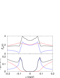
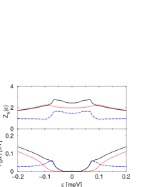
Figure 15: The different contributions to the renormalization factor (top) and the scattering rate (bottom) are shown for the $M$ point (left) and for the $N$ (node) point (right). Dotted curves are the contribution from the spin fluctuation continuum, dashed the contribution from the spin fluctuation mode, and full both contributions.

Finally, note that in the normal state, the even channel stays gapped. That means that at the $N$ point, the self energy for scattering between bonding bands and between antibonding bands (but not between bonding and antibonding) is similar to one half the continuum contribution (dotted line) in the right panel of Fig. 15. This will induce a weaker kink feature in the normal state at an energy equal to the even channel (optical) gap in the spin susceptibility, which is around 50-60 meV. Correspondingly, the high energy renormalization will be present in the normal state, but weaker. The difference between the high energy renormalization in the normal and superconducting states is mainly due to the appearance of a continuum gap in the odd channel. The low energy renormalization is mainly due to the appearance of the mode in the odd channel.

III.4 Renormalization of EDC and MDC dispersions

In the following, we discuss the dispersion of the spectral lineshape through the Brillouin zone and study the corresponding EDC (as determined from the spectral maximum as a function of energy) and MDC (as determined from the spectral maximum as a function of momentum) dispersions. We include both the mode and the gapped continuum of the spin fluctuation spectrum. In Figs. 16-19, we show dispersions of the ARPES spectra along several selected paths in the Brillouin zone. In the left panels of the figures, the intensities and spectral lineshapes can be followed, and in the right panels, the corresponding dispersions of the peak maxima and hump maxima in the EDCs are shown as circles, and the maxima in the corresponding MDC dispersions as curves. A general remark concerns the linewidth of the high energy features compared to the low energy features. Due to the strong self energy damping effects setting in above the dip energy (Fig. 15), the hump features are considerably broader than the peak features for all momenta in the Brillouin zone. This holds for both EDC and MDC dispersions. Note that even without taking into account the lifetime effects due to the spin fluctuation continuum, the high energy features are much broader in energy than the low energy features.Eschrig00 To account for the experimental MDC linewidth, however, one has to take into account the continuum contribution.

Starting with Fig. 16, we follow the dispersion along a cut going from the $M$ point of the Brillouin zone towards the $Y$ point. The $A$ point corresponds to spectra roughly in the middle of the set. From the left panel, we see that sharp peaks are restricted to the momentum regions between the $M$ and $A$ points. The dip structure is maximal at the $M$ point and much weaker at the $A$ point. The corresponding dispersion, shown in the right panel, reproduces the experimental findingsKaminski00 of two almost dispersionless EDC branches, one for the peak and one for the hump. The MDC follows the peak branch, then shows a nontrivial variation at energies within the gap edge. This behavior is discussed in Ref. Norman01a, . The Fermi crossing is only slightly shifted with respect to the unrenormalized value of $k_{x}=0.18\pi$. At higher energies, the MDC is peaked at $M$.

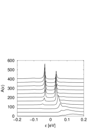
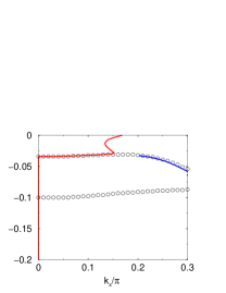
Figure 16: Left: Dispersion of the spectral intensity and lineshape as a function of momentum along the $M-Y$ cut, ($k_{y}=\pi$, $k_{x}=0...0.4\pi$ in steps of $0.04\pi$ from top to bottom). Right: EDC (circles) and MDC (curve) dispersions from maxima of the curves shown in the left panel. In the EDC dispersion, the low energy peak and the high energy hump with the break feature in between is clearly visible. Because the bottom of the normal state dispersion is at $\xi_{M}=-34$meV, the MDC shows only a broad maximum at $M$ for high energies.

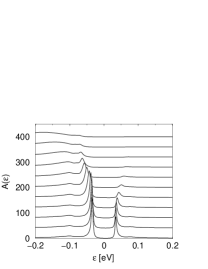
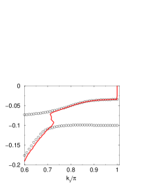
Figure 17: Left: Dispersion of the spectral intensity and lineshape as a function of momentum along the $M-\Gamma$ cut ($k_{x}=0$, $k_{y}=0.6\pi..\pi$ in steps of $0.04\pi$ from top to bottom). Right: EDC (circles) and MDC (curve) dispersions from maxima of the curves shown in the left panel.

Going from the $M$ point in the direction of the $\Gamma$ point, the corresponding dispersion of the ARPES spectra is shown in Fig. 17. On the left side, one can see that the intensity of both the peak and the hump is almost unaffected in the region between the $M$ point and roughly $0.3\pi$ from there in direction of $\Gamma$. In this range, the renormalized EDC dispersion of the hump is extremely flat, as seen in the right panel, and the peak shows a moderate dispersion, becoming almost flat between $q_{y}=0.9\pi$ and $q_{y}=\pi$. When going further away from the $M$ point, the intensity of the peak drops sharply, and a strong dispersion of the hump sets in. There is a clear break between the peak and the hump EDC dispersion due to the dip. The MDC along this cut follows the peak near the $M$ point, but changes over to the hump dispersion at roughly the point where the hump starts to disperse strongly away from the chemical potential. In this range, at energies between 70 meV and 100 meV, the MDC dispersion is almost vertical, with a weak S-like shape. We draw the attention to the fact that the hump shows a weakly positive dispersion close to the $M$ point, with point of closest approach to the chemical potential at $q_{y}\approx 0.85\pi$. This effect is due to the coupling of the $(\pi,0)$ and $(0,\pi)$ points by self energy effects, and is a result of the fact that going towards $\Gamma$ from the $(\pi,0)$ point means going towards $Y$ from the $(0,\pi)$ point at the $(\pi,\pi)$-displaced wavevector. As a result of this, the weakening of the self energy effect along the $M-\Gamma$ cut leads to a minimum in the hump dispersion at the $M$ point. This effect was experimentally found.Campuzano99

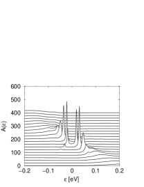
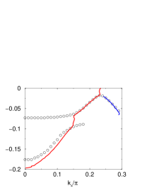
Figure 18: Left: Dispersion of the spectral intensity and lineshape as a function of momentum $k_{y}=0.6\pi$, $k_{x}=0...0.4\pi$ in steps of $0.02\pi$ from top to bottom. Right: EDC (circles) and MDC (curve) dispersions from maxima of the curves shown in the left panel.

In Fig. 18, we show our results for a cut parallel to the $M-Y$ cut shown in Fig. 16, keeping $q_{y}=0.6\pi$ constant. At low energies, the spectral evolution, seen on the left part of the figure, shows the typical BCS mixing between particle and hole states. Concentrating on the negative energy parts, again two branches are present, the peak branch and the hump branch, separated by a break in the EDC dispersion. Both branches now show considerable dispersion, but still overlap in momentum. The MDC dispersion changes from the low energy peak branch to the high energy hump branch at roughly the point where the intensity of the peak drops dramatically. Note that the EDC and MDC dispersions are considerably displaced relative to one another at high energies. Also at low energies, the MDC dispersion is stronger near the break region than the EDC dispersion. This effect increases when the residual width of the quasiparticle peak increases, and when convolution with the experimental resolution function is taken into account.Norman01a

Finally, we discuss the cut along the nodal direction, shown in Fig. 19. For this direction, the gap is zero as a consequence of $d$ wave symmetry, and as a result the EDC dispersion should cross the Fermi energy. This is seen in the left panel of the figure. Note the very strong damping of the spectral peak as soon as it crosses the energy region which corresponds to the break effect near the $M$ point. Actually, the damping starts at slightly lower energies, due to the onset of node-node scattering processes at an energy $\Omega_{res}$, as can be seen in the left panel of Fig. 19. The velocity renormalization for low energies and high energies differs by a factor of roughly two, both for EDCs and MDCs, in agreement with experiment.Kaminski00 Finally, we also reproduce the experimental fact that the high energy dispersion does not extrapolate to the Fermi crossing.Bogdanov00 ; Lanzara01 Again, note some shift between the EDC and MDC dispersions at high energies due to the energy variation of the self energy.

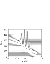
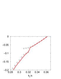
Figure 19: Left: Dispersion of the spectral intensity and lineshape in the nodal direction ($\Gamma-Y$) as a function of momentum $k_{x}=k_{y}=0.25\pi...0.45\pi$ in steps of $0.01\pi$ from top to bottom. Right: the corresponding EDC (circles) and MDC (curve) dispersions. The kink is most clearly seen in the MDC dispersion. The low energy velocity is roughly half the high energy one. The high energy dispersion does not extrapolate to the Fermi surface crossing.

Clearly, the velocity break (kink) along the nodal direction and the break between the peak and hump (dip) near the $M$ point are occurring in the same energy range between $-\Omega_{res}-\Delta_{A}$ and $-\Omega_{res}-E_{M}$. This is an appealing result of our theory, because it explains all features in the dispersion anomalies in the Brillouin zone seen by ARPES with a simple model.

III.5 Tunneling spectra

Knowing the spectral function, $A(\epsilon,\vec{k})$, throughout the zone, we are able to calculate the tunneling spectra given a tunneling matrix element $T_{\vec{k}\vec{p}}$. For simplicity, we present numerical results for the simple model, neglecting the continuum part of the spin fluctuation spectrum. From the SIN tunneling current $I(V)$, one obtains the differential conductance, $dI/dV$. As usual, we neglect the energy dependence of the SIN matrix element $|M_{\vec{k}}|^{2}=2e\sum_{\vec{p}}|T_{\vec{k}\vec{p}}|^{2}A_{N}(\vec{p},\epsilon)$, where $A_{N}$ is the spectral function of the normal metal. The SIN tunneling current is then given by

$$I(V)=\sum_{\vec{k}}|M_{\vec{k}}|^{2}\int_{-\infty}^{\infty}\frac{d\epsilon}{2\pi}A(\epsilon,\vec{k})\left\{f(\epsilon)-f(\epsilon+eV)\right\}$$ (38)

We model the tunneling matrix element for two extreme cases: for incoherent tunneling we assume a constant $|M_{\vec{k}}|^{2}=M_{0}^{2}$, whereas for coherent tunneling we use $|M_{\vec{k}}|^{2}=\frac{1}{4}M_{1}^{2}(\cos k_{x}-\cos k_{y})^{2}$. Chakravarty93 Coherent tunneling in the c-axis direction is strongly enhanced for the $M$ points in the Brillouin zone compared to the regions near the zone diagonal due to the matrix elements.Chakravarty93 Our numerical results for SIN junctions are shown in Fig. 20 (left). In both cases, we observe a clear asymmetry, with a dip-hump structure on the negative bias side and a very weak feature on the positive side of the spectrum, as in experiments.Renner95 ; DeWilde98 The low energy behavior of the tunneling spectrum in the coherent tunneling limit does not show the characteristic linear in energy behavior for $d$-wave, because the nodal electrons have suppressed tunneling as a result of the matrix elements. The peak-dip-hump features, on the other hand, are not affected by the matrix elements, as they are dominated by the $M$ point regions which are probed by both coherent and incoherent tunneling.

For an SIS junction, the single particle tunneling current is given in terms of the spectral functions by

$$I(V)=2e\sum_{\vec{k}\vec{p}}|T_{\vec{k}\vec{p}}|^{2}\int_{-\infty}^{\infty}\frac{d\epsilon}{2\pi}A(\epsilon,\vec{k})A(\epsilon+eV,\vec{p})$$

$$\times\left\{f(\epsilon)-f(\epsilon+eV)\right\}$$ (39)

Again we show results for incoherent tunneling ($|T_{\vec{k}\vec{p}}|^{2}=T_{0}^{2}$) and for coherent tunneling with conserved parallel momentum, $|T_{\vec{k}\vec{p}}|^{2}=\frac{1}{16}T_{1}^{2}(\cos k_{x}-\cos k_{y})^{4}\delta_{\vec{k}_{||},\vec{p}_{||}}$.Chakravarty93 Our results are shown in the right panel of Fig. 20.

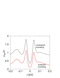
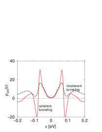
Figure 20: Differential tunneling conductance for SIN (left) and SIS (right) tunnel junctions for $T=40$ K. Units are $eM_{i}^{2}$ for SIN and $2e^{2}T_{i}^{2}$ for SIS. Results for the coherent (full curves) and incoherent (dashed curves) tunneling limits are shown. The parameters are given in Table 2.

All structures are symmetric around the chemical potential. The low energy part of the spectrum is strongly suppressed in the incoherent tunneling limit already, thus there is no big difference to the coherent tunneling limit there. At higher voltages, however, in the coherent tunneling limit, we obtain negative differential conductance. Such an effect was observed recently in optimally doped Bi₂Sr₂CaCu₂O_8-δ break junctions.Zasadzinski01 We also observe negative behavior at higher bias in the coherent tunneling limit, but note that in reality, the tunneling matrix element will have both coherent and incoherent contributions (especially at higher voltages), and thus will be a weighted average of the dashed and full curves in Fig. 20. In this case, most probably only the negative behavior below 100 meV will be observable. We note that the spin fluctuation continuum broadens the spectral functions and, as we show below, this leads to a positive response at higher voltages.

We give approximate expressions for the SIS differential conductances for zero temperature. In the incoherent limit,

$$I^{(incoh)}(V)=\frac{eT_{0}^{2}}{\pi}\int_{-eV}^{0}d\epsilon N(\epsilon)N(\epsilon+eV)$$ (40)

In the coherent tunneling limit, the tunneling matrix element very effectively suppresses the nodal regions, thus only allowing for tunneling near the $M$ point regions. In these regions, however, the dispersion is weak, so that we may approximate the spectral function by its value at the $M$ point, $A_{M}(\epsilon)$. Then, we obtain in the coherent tunneling limit

$$I^{(coh)}(V)\approx\frac{eT_{1}^{2}}{\pi}\int_{-eV}^{0}d\epsilon A_{M}(\epsilon)A_{M}(\epsilon+eV)$$ (41)

with $T_{1}^{2}=\sum_{\vec{k}\vec{p}}|T_{\vec{k}\vec{p}}|^{2}$. Note that two different quantities are probed in the two limits. In the incoherent limit, it is the density of states, and in the coherent limit, it is the spectral function at the $M$ point of the Brillouin zone.

It is easy to show by differentiating Eq. 41 that the differential conductance can be negative, and furthermore, can approach a negative value for large voltages. The limiting behavior at high voltages in the incoherent tunneling limit is proportional to $N(-)N(+)$, where $N(\pm)$ is the density of states at large positive/negative energies. If in the coherent tunneling limit the corresponding term proportional to $A_{M}(+)A_{M}(-)$ is very small, then the main contribution comes from the region where either $\epsilon\approx-\Delta_{M}$ or $\epsilon+eV\approx\Delta_{M}$, varying within a range of order $\Delta_{M}$ around these values. It is easy to show that this contribution is negative. But as soon as incoherent contributions play any role, or if $A_{M}$ has a considerable incoherent part, then their positive contributions will dominate at high voltages. Note that for SIN tunneling, the differential conductance is always positive definite.

III.6 Self consistency issues

When going towards underdoping, the spectral function deviates considerably from the bare BCS spectrum. Self consistency issues become important then.

Our studies have shown that the quasiparticle peak is always reasonably well separated in energy from the high energy incoherent part by a dip. By coupling electrons to the spin resonance mode, weight is shifted from the quasiparticle peak to the incoherent part which includes the broad hump structure. Thus, when calculating the self energy effects due to this coupling, only the quasiparticle peak part of the spectrum with its reduced weight will contribute to the sharp self energy features at energies affecting the quasiparticle peak. The incoherent part of the fermionic spectrum, which is gapped by roughly the hump energy, will affect the low energy quasiparticle properties only in form of an effective high energy renormalization factor, which is constant up to energies comparable to the hump energy. This effective renormalization adds to the one due to coupling of electrons to the spin fluctuation continuum. Thus, we can concentrate on the renormalization equations following from the set of equations which includes the quasiparticle peak spectrum of reduced weight interacting with the spin fluctuation mode. In deriving these equations, we make use of the approximate equations for the renormalization functions derived above.

The quasiparticle part of the Green’s function has in this approximation at the $M$ point the form

$$G^{R}_{\epsilon,k_{M}}=\frac{1}{\tilde{Z}_{M}}\left(\frac{\tilde{A}^{+}_{M}}{\epsilon-\tilde{E}_{M}+i\tilde{\Gamma}_{M}}+\frac{\tilde{A}^{-}_{M}}{\epsilon+\tilde{E}_{M}+i\tilde{\Gamma}_{M}}\right)$$ (42)

$$F^{R}_{\epsilon,k_{M}}=\frac{1}{\tilde{Z}_{M}}\left(\frac{\tilde{C}_{M}}{\epsilon-\tilde{E}_{M}+i\delta_{M}}-\frac{\tilde{C}_{M}}{\epsilon+\tilde{E}_{M}+i\delta_{M}}\right)$$ (43)

where $\tilde{E}_{M}=\sqrt{\tilde{\xi}_{M}^{2}+\tilde{\Delta}_{M}^{2}}$ and $\tilde{A}^{\pm}_{M}=(1\pm\tilde{\xi}_{M}/\tilde{E}_{M})/2$. Here, $\tilde{E}_{M}$ is the measured peak position at the $M$ point, and $\tilde{\Gamma}_{M}$ is the quasiparticle peak width. The broadening of the off-diagonal spectra, $\delta_{M}$, is reduced compared to $\tilde{\Gamma}_{M}$ due to $d$-wave symmetry. Using the approximative formulas from the last sections at $\epsilon=-\tilde{E}_{M}$, we obtain (with $\alpha=g^{2}I_{0}/\pi$)

$$\tilde{Z}_{M}=1+\frac{\lambda_{M}^{(N)}}{\tilde{Z}_{N}}+\lambda_{M}^{(c)}+\frac{\alpha}{\tilde{Z}_{M}\Omega_{res}\tilde{E}_{M}}\frac{\tilde{E}_{M}}{\Omega_{res}+2\tilde{E}_{M}}$$ (44)

$$\tilde{\Delta}_{M}=\frac{\Delta_{M}}{\tilde{Z}_{M}}+\frac{\alpha}{\tilde{Z}_{M}^{2}\Omega_{res}\tilde{E}_{M}}\frac{\Omega_{res}+\tilde{E}_{M}}{\Omega_{res}+2\tilde{E}_{M}}\tilde{\Delta}_{M}$$ (45)

$$\tilde{\xi}_{M}=\frac{\xi_{M}}{\tilde{Z}_{M}}-\frac{\alpha}{\tilde{Z}_{M}^{2}\Omega_{res}\tilde{E}_{M}}\frac{\Omega_{res}+\tilde{E}_{M}}{\Omega_{res}+2\tilde{E}_{M}}\tilde{\xi}_{M}$$ (46)

where $\lambda_{M}^{(c)}$ denotes renormalizations due to the spin fluctuation continuum and the incoherent part of the spectral function, and $\lambda_{M}^{(N)}$ the contribution coming from the nodal regions (these contributions are renormalized with the nodal renormalization factor $\tilde{Z}_{N}$, which is smaller than $\tilde{Z}_{M}$). The last two equations merely express the measurable quantities $\tilde{\Delta}_{M}$ and $\tilde{\xi}_{M}$ as functions of the bare quantities $\Delta_{M}$ and $\xi_{M}$. The first equation can be solved, giving for small $\Omega_{res}$ and not too small $g^{2}I_{0}$ a quasiparticle weight $\propto\sqrt{\Omega_{res}(\Omega_{res}+2\tilde{E}_{M})}$. Note that we derived this set of equations for the case where $\tilde{\Gamma}_{M}$ is neglected, which describes the slightly underdoped region. When $\Omega_{res}$ becomes comparable to $\tilde{\Gamma}_{M}$, these equations have to be modified.

It should be remarked, though, that using these equations in the absence of vertex corrections usually give poorer results than those presented in this paper using bare Green’s functions.Vilk97

III.7 Bilayer splitting

For bilayer compounds, the dispersion can be split into bonding ($b$) and antibonding ($a$) bands. Accordingly, the self energy for each band is defined as $\Sigma_{k,\epsilon}^{(b)}$ and $\Sigma_{k,\epsilon}^{(a)}$. Similarly, the spin susceptibility is now a matrix in the bonding-antibonding indices, having elements diagonal ($\chi_{aa}$, $\chi_{bb}$) and off-diagonal $(\chi_{ba}$, $\chi_{ab}$) in the bonding-antibonding representation. The components of the spin susceptibility transforming even and odd with respect to the plane indices are given by $\chi_{e}=\chi_{aa}+\chi_{bb}$ and $\chi_{o}=\chi_{ab}+\chi_{ba}$. For identical planes, we have $\chi_{aa}=\chi_{bb}$ and $\chi_{ab}=\chi_{ba}$. The measured susceptibility is then given by

$$\chi=\chi_{e}\cos^{2}\frac{q_{z}d}{2}+\chi_{o}\sin^{2}\frac{q_{z}d}{2}$$ (47)

where $d$ is the separation of the layers within a bilayer. If we write the self energy for a single layer as $\chi\ast\hat{G}$ (the hat denotes the 2x2 particle hole space), which is a functional of the spin susceptibility $\chi$ and the Gor’kov-Green’s function $\hat{G}$, then we have formally for the two-layer system

$$\hat{\Sigma}^{(b)} = \chi_{e}\ast\hat{G}^{(b)}+\chi_{o}\ast\hat{G}^{(a)}$$

$$\hat{\Sigma}^{(a)} = \chi_{e}\ast\hat{G}^{(a)}+\chi_{o}\ast\hat{G}^{(b)}$$ (48)

For the resonance part, which only has a $\chi_{o}$ component, this means that fermionic excitations of the antibonding band determine the self energy for the bonding band and vice versa. The calculations presented in this paper hold for the case of bilayer systems if we assume identical dispersions for bonding and antibonding bands. Even small bilayer splittings of the order of 10 meV or less do not matter, as they do not qualitatively alter the spectral form of the self energy. For larger bilayer splittings, the self energy is larger for the bonding band, because it is determined by the van Hove singularity near the chemical potential in the antibonding band. Thus, stronger renormalizations are expected in the bonding band for this case, which tends to decrease the bonding-antibonding splitting. This effect of reducing the bilayer splitting should be strongest in underdoped compounds, where the effect of the resonance mode is strongest. In overdoped compounds, the bilayer splitting should be less affected by spin fluctuations. Our prediction is that if a bilayer splitting is observed, then the peak-dip-hump structure should be stronger for the bonding band with the higher binding energy peak. This is consistent with the data of Ref. Feng01a, . The onset of strong fermionic damping should be independent of the band index, as it is given by scattering to the nodes, and thus occurs at the fixed energy $\Omega_{res}$.

In this paper, we have elected not to explicitly include bilayer splitting effects in our calculations. The primary reason is that although all ARPES groups now detect the presence of bilayer splitting for heavily overdoped samples, the various groups disagree on its presence for optimal and underdoped samples Kaminski02 . Recently, we have performed calculations including bilayer splitting and are able to reproduce a number of unusual spectral anomalies seen in heavily overdoped ARPES spectra Eschrig02 . These calculations further confirm the picture advocated in this paper, in that the spectral anomalies imply a mode which has odd symmetry with respect to the layer index of the bilayer, a unique property of the magnetic resonance observed by neutrons. For further details, the reader is referred to Ref. Eschrig02, .

III.8 Doping dependence

In this section, we deal with the doping dependence of the spectral lineshape near the $M$ point of the Brillouin zone. As there are many parameters which change with doping in different ways, it could turn out to be a meaningless task to adjust all of those parameters and at the same time make a sensible prediction. But, fortunately, all changes with doping lead to spectral changes which go in the same direction. This ‘fortuitous’ accident allows us to make some general predictions from the theory we use. To see this, we turn again to Figs. 11 and 12. From there we see that the quasiparticle weight decreases with decreasing $\Omega_{res}/\Delta_{M}$, and with increasing coupling constant $g^{2}w_{Q}$. The quasiparticle scattering rate increases with decreasing $\Omega_{res}/\Delta_{M}$. And the hump energy disperses to higher binding energies for increasing coupling constant and increasing $\xi_{M}$. Thus, in our model, going from overdoping to underdoping amounts to a decreasing quasiparticle weight, an increasing quasiparticle scattering rate, and an increasing hump binding energy.

The important parameter, as we see from this study, is the ratio $\Omega_{res}/\Delta_{M}$, the ratio of the mode energy to the maximal superconducting $d$-wave gap. We distinct two regions: the first, where $\Omega_{res}/\Delta_{M}>1$, and the second, where $\Omega_{res}/\Delta_{M}<1$. The situation is schematically shown in the phase diagram in Fig. 21. The curves shown are calculated using the formulas (we relate $T_{c}$ to the hole doping level in the Cu-O₂ planes in the usual mannerPresland91 )

$$T_{c} = 95\mbox{ K}\left(1-82.6(p-0.16)^{2}\right)$$ (49)

$$\Delta_{M} = 38\mbox{ meV}\left(1-9.1(p-0.16)\right)$$ (50)

$$\Omega_{res} = 40\mbox{ meV}\left(1-82.6(p-0.16)^{2}\right)$$ (51)

All these quantities approach zero on the overdoped side at $p=0.27$. Optimal doping corresponds to $p=0.16$. Note that $\Omega_{res}=4.9T_{c}$ in agreement with Ref. Zasadzinski01, . The $\Delta_{M}$ variation was based on ARPES data.Campuzano99 ; Mesot99

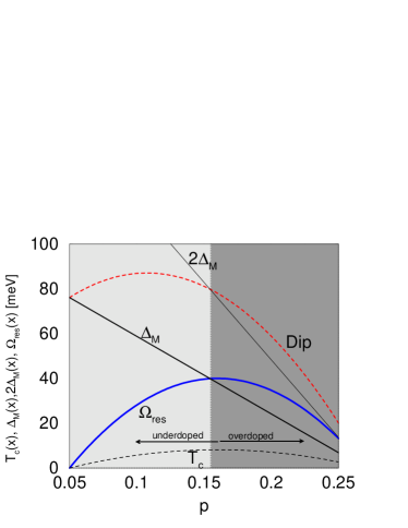
Figure 21: In the dark gray shaded region, corresponding to overdoping, quasiparticles peaks are well defined. In the light gray shaded region, corresponding to underdoping, the peak weight is strongly reduced, and an incoherent part due to scattering from the spin fluctuation mode is dominant. The resonance energy, shown as a thick line, is bounded from above by twice the maximal gap energy, $\Omega_{res}<2\Delta_{M}$, and approaches it on the overdoped side. The position of optimal doping, at maximal $T_{c}$ and $\Omega_{res}$, roughly coincides with the point where $\Delta_{M}$ as a function of doping crosses $\Omega_{res}$.

As can be seen, the separation between overdoped and underdoped regions roughly coincides with the regions where $\Omega_{res}>\Delta_{M}$ and $\Omega_{res}<\Delta_{M}$, respectively. The dip onset is given by $\Omega_{res}+\Delta_{A}$. As $\Delta_{A}$ is about the same as $\Delta_{M}$, we have shown in Fig. 21 the line for $\Omega_{res}+\Delta_{M}$ as a dashed line, which determines the position of the dip fairly accurately. The continuum in the spin fluctuation spectrum only affects electrons above $2\Delta_{h}$, which is near or above the dip energy. One important observation is that the point of optimal doping for a Cu-O₂ plane roughly corresponds to the point where $\Omega_{res}/\Delta_{M}=1$. Thus, region I of Fig. 5 is relevant to overdoped materials, and region II to underdoped materials. Another experimental observation is that this ratio never exceeds the value two. This is expected for an excitonic collective mode below a continuum edge.Zasadzinski01

For a quantitative theory of the doping dependence the self consistency issue becomes important. The coherent quasiparticle weight and the quasiparticle linewidth are given by,

$$z_{M}\approx\frac{1}{\tilde{Z}_{M}}\left(\frac{1}{2}+\frac{|\tilde{\xi}_{M}|}{2\tilde{E}_{M}}\right)$$ (52)

$$\tilde{\Gamma}_{M}\approx\frac{g^{2}w_{MN}}{\pi\tilde{v}_{N}\tilde{v}_{\Delta}}\frac{\tilde{E}_{M}-\Omega_{res}}{\tilde{Z}_{M}}\Theta(\tilde{E}_{M}-\Omega_{res})$$ (53)

where $\tilde{Z}_{M}\equiv\tilde{Z}_{M}(-\tilde{E}_{M})$ is the only quantity not available from experiment. We can eliminate it, to obtain the relation

$$\tilde{\Gamma}_{M}\approx 2z_{M}\tilde{E}_{M}\frac{g^{2}w_{MN}}{\pi\tilde{v}_{N}\tilde{v}_{\Delta}}\frac{\tilde{E}_{M}-\Omega_{res}}{\tilde{E}_{M}+|\tilde{\xi}_{M}|}\Theta(\tilde{E}_{M}-\Omega_{res})$$ (54)

Note that experimentally both $z_{M}\tilde{E}_{M}$ and (possibly) $\tilde{v}_{\Delta}$ scale with $k_{B}T_{c}$.Ding00 ; Mesot99 So, the quasiparticle width is dominated by the difference $\tilde{E}_{M}-\Omega_{res}$. Quasiparticles are sharp at the overdoped side where $\tilde{E}_{M}<\Omega_{res}$, and an onset of quasiparticle scattering as a function of underdoping takes place when $\tilde{E}_{M}=\Omega_{res}$. This point is slightly beyond optimal doping.

IV Coupling to the zone boundary half breathing optical phonon

The sharp structure in the dispersion needs an explanation in terms of an almost dispersionless feature which couples to the electrons. Numerous phonons modes are seen in inelastic neutron scattering in high $T_{c}$ cuprates. Most of them do not show indications of strong coupling to electrons. Two special types of phonons have attracted attention: the Cu-O buckling mode, which is attractive in the $d$-wave channel,Song95 ; Nazarenko96 ; Bulut96 ; Dahm96 ; Sakai97 ; Nunner99 and the Cu-O breathing mode, which is repulsive in the $d$-wave channel.Nazarenko96 ; Bulut96 ; Dahm96 ; Nunner99 Typically, the absolute values of the pairing interactions in the $B_{1g}$ (‘$d$-wave’) channel for both types of vibrations are smaller than 0.1 eV, in the $A_{1g}$ (‘$s$-wave’) channel about 0.5-1 eV; for spin fluctuations, the corresponding numbers are in the $d$-wave channel 0.5-1 eV and in the $s$-wave channel 1-2 eV.Nunner99 The total electron-phonon coupling constant in the $s$-wave channel amounts to $\lambda_{s}\approx 0.4-0.6$,Friedl90 ; Litvinchuk91 ; Andersen96 ; Jepsen98 ; Nunner99 and in the $d$-wave channel to $\lambda_{d}\approx 0.3$.Andersen96 ; Jepsen98 Thus, phonons are not likely to be responsible for the high transition temperature.

It was argued recently that strong coupling of electrons to the zone boundary half breathing phonon may be responsible for the anomalies in the dispersion. It is known for some time that this phonon shows a dispersion which is strongly renormalized midway between the zone boundary and the zone center when entering the superconducting state. These findings show that the zone boundary half breathing phonon is affected by superconductivity. It was suggested to be responsible for the renormalizations of the dispersion observed in ARPES.Lanzara01 This zone boundary half breathing longitudinal optical phonon is a Cu-O bond stretching mode with an energy between 50 and 100 meV. Its dispersion is very strong in the middle of the branch, and it was suggested that a discontinuity develops there in the metallic state.McQueeney99 The first measurements concentrated on lanthanum cuprates, but recently YBa₂Cu₃O_7-δ was also studied.Petrov00 ; McQueeney01 The displacements involve oscillations of the oxygen atoms in phase between the two planes in the bilayer. The results for optimally doped YBa₂Cu₃O_7-δ are the following: The dispersion of the zone edge mode in the superconducting state shows a ‘break’ at $(0,\pi/2)$ (and equivalent points), with an almost dispersionless branch (at $\sim 55$ meV) between $\vec{q}=(0,\pi/2)$ and $\vec{q}=(0,\pi)$, and a dispersive branch (68 meV to 72 meV) between $\vec{q}=(0,0)$ and $\vec{q}=(0,\pi/2)$.McQueeney99 ; Petrov00 ; McQueeney01 Experimental investigation showed that the dispersionless branch extends over a region $\pi/2<q_{x}<\pi,-0.1\pi<q_{y}<0.1\pi$ (and analogously for $q_{x}$ and $q_{y}$ interchanged).McQueeney99 The dispersionless branch was only observed for bond stretching along the $a$ direction (perpendicular to the chains). The dispersions of the longitudinal bond-stretching phonon branches were found to show no apparent temperature dependence.McQueeney01 The phonon intensity was found to show significant temperature dependence below $T_{c}$.Petrov00 Phonon weight is transferred from a position halfway to the zone boundary (in a range between 55 meV and 70 meV) to the zone center (70-75 meV) and the zone boundary (50-55 meV). This transfer sets in at $T_{c}$ and increases with decreasing temperature.

The coupling strength, $g_{b}(\vec{q})$, goes to zero for small momentum transfer $\vec{q}$. Furthermore, in the model of Ref. Shen01, , the coupling vanishes near the $\vec{q}=(\pi,\pi)$ point, thus having minimum impact on the electrons near the $M$ point of their Brillouin zone. This is in stark contrast to the resonance mode model, and can certainly not explain the effects at the $M$ points. It is, however, possible that they contribute to the renormalization of the nodal dispersion. The maximal coupling strength was theoretically estimated to $g_{b}\approx 0.04$eV,Nunner99 , but in some models is enhanced by vertex corrections.Shen01

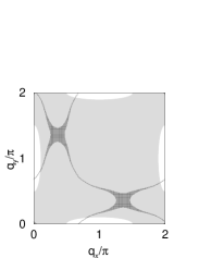
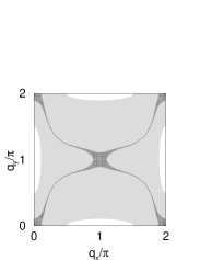
Figure 22: As in Figs. 3 d) and 4, but the white areas now denote the experimentally determined regions where the dispersionless half breathing zone boundary phonon mode is present. For nodal wave vectors (left) the main self energy contribution comes from node-node scattering processes at small energies (near $-\Omega_{phon}$). At the $M$ point (right) the self energy effects are negligible due to geometric restrictions. Only higher anharmonic terms (with two phonon processes which add up to a $(\pi,\pi)$ wavevector) could contribute at fermionic wavevectors near the $M$ point.

In Fig. 22, we point out an important difference to the magnetic mode. The magnetic mode is peaked around $(\pi,\pi)$, whereas the spectral density of half breathing phonon is peaked around the points $(0,\pi)$ and $(\pi,0)$. Because for the imaginary part of the self energy only excitations near the Fermi surface are important, there are geometric restrictions for the possible scattering events. In the case of the magnetic mode, scattering was dominated by processes connecting the $M$ points of the Brillouin zone, and these scattering processes are enhanced by the presence of a van Hove singularity close to the chemical potential. In the case of the half breathing phonon, the $M$ point electrons are very ineffectively scattered by these phonons due to the Pauli exclusion principle. The important points here are near the nodal regions for the electrons. Thus, the strongest effects are expected near (but not necessarily at) the nodes, not near the $M$-points, in contrast to what experiment shows.

It is possible that both processes play a role and dominate in different regions of the Brillouin zone. Phonons would then play some role for nodal electrons.

V Conclusions

We suggest that the van Hove singularity at the $M$ point of the Brillouin zone plays an important role in determining the self energy effects observed in ARPES and tunneling experiments. The picture can be understood as follows: the quasiparticle dispersion is fairly flat near the $M$ points of the Brillouin zone, with a large effective mass in the $M-\Gamma$ direction, and is close to the chemical potential. Because the continuum part of the spin fluctuation spectrum is gapped up to energies $\sim 70$ meV, the scattering at low energies is dominated by scattering processes accompanied by emission of a spin fluctuation mode (which lies below the gapped continuum at $\sim 40$ meV and has a sharp energy). This coupling leads to cusps in the energy dependence of the self energy in the range of 70-80 meV due to the effect of the van Hove singularities at the $M$ and $A$ points. Because of the finite width of the spin fluctuation mode in momentum, there are traces of these cusps for electrons at all positions near the Fermi surface. The position in energy of these cusps are determined by electrons near the $M$ and $A$ points only, which explains the isotropy around the Fermi surface of the energy scale of 70-80 meV where kink features in the dispersion are observed. The intensity of this self energy effect is determined by the intensities of the spin fluctuation mode at such momenta $\vec{q}$ which connect the electron with momentum $\vec{k}$ to electrons near the $M$ point region. Thus, $\vec{q}=(\vec{k}-\vec{k}_{M})$ modulo $(\vec{G})$, where $\vec{G}$ is a reciprocal lattice vector. This intensity is large for $\vec{k}\approx\vec{k}_{M}$, but smaller for $\vec{k}\approx\vec{k}_{N}$. This explains the strong anisotropy of the magnitude of the effect around the Fermi surface.

VI Acknowledgements

We would like to thank Adam Kaminski and Juan Carlos Campuzano for discussions concerning their photoemission data, and John Zasadzinski concerning tunneling data. We acknowledge communications with Steve Kivelson and Hae-Young Kee, and helpful discussions with Andrey Chubukov. This work was supported by the U. S. Dept. of Energy, Office of Science, under Contract No. W-31-109-ENG-38.

Note added in proof. After submitting this paper, we became aware of an experimental paper which claims no momentum anisotropy in the linewidth for overdoped compounds Bogdanov02 . This result is actually consistent with our picture, in that for overdoped compounds, the spectral peak lies inside the scattering rate gap, which can be appreciated from Fig. 21.

Appendix A Self energies

In this appendix, we derive self energy expressions which allow us to evaluate the real part of the self energy analytically in several special cases, and have the numerical advantage of having eliminated all principal value integrals. The procedure is a generalization of a method developed by F. Marsiglio et al.Marsiglio88 The self energy is given by,

$$\Sigma^{R}_{\epsilon,k}=\frac{i}{2}g^{2}\sum_{q,\omega}\left(G^{R}_{\epsilon-\omega,k-q}D^{K}_{\omega,q}+G^{K}_{\epsilon-\omega,k-q}D^{R}_{\omega,q}\right)$$ (55)

where $D=-\chi$. In equilibrium, the Keldysh components are given by the simple expressions

$$D^{K}_{\omega,q}=\left(D^{R}_{\omega,q}-D^{A}_{\omega,q}\right)\coth\frac{\omega}{2T}=-iB_{\omega,q}(1+2b_{\omega})\quad$$ (56)

$$G^{K}_{\epsilon,k}=\left(G^{R}_{\epsilon,k}-G^{A}_{\epsilon,k}\right)\tanh\frac{\epsilon}{2T}=-iA_{\epsilon,k}(1-2f_{\epsilon})\quad$$ (57)

where $B_{\omega,q}$ and $A_{\epsilon,k}$ are the bosonic and fermionic spectral functions, and $b_{\omega}$, $f_{\epsilon}$ their corresponding distribution functions, respectively. Note, that the Keldysh components are purely imaginary.

In evaluating these integrals, the only numerical complication comes from the real parts of $\Sigma$ due to principal value integrals. We can eliminate those by using the following trick: Note that in equilibrium the identities

$$\sum_{\omega}D^{R}_{\omega}G^{K}_{\epsilon-\omega}=-i\sum_{\omega}\tanh\frac{\epsilon-\omega}{2T}B_{\omega}G^{R}_{\epsilon-\omega}$$

$$\quad+\sum_{\omega}\left(D^{A}_{\omega}G^{R}_{\epsilon-\omega}-D^{R}_{\omega}G^{A}_{\epsilon-\omega}\right)\tanh\frac{\epsilon-\omega}{2T}$$ (58)

$$\sum_{\omega}D^{K}_{\omega}G^{R}_{\epsilon-\omega}=-i\sum_{\omega}\coth\frac{\omega}{2T}D^{R}_{\omega}A_{\epsilon-\omega}$$

$$\quad+\sum_{\omega}\left(D^{R}_{\omega}G^{A}_{\epsilon-\omega}-D^{A}_{\omega}G^{R}_{\epsilon-\omega}\right)\coth\frac{\omega}{2T}$$ (59)

hold which are easy to check. The convenient feature is that the second lines in Eqs. A and A can be converted into Matsubara sums by noting that $D^{A}_{\omega}G^{R}_{\epsilon-\omega}$ is an analytic function in the lower $\omega$ half plane, and analogously $D^{R}_{\omega}G^{A}_{\epsilon-\omega}$ analytic in the upper half plane. Thus,

$$\frac{i}{2}\sum_{\omega}\left(D^{A}_{\omega}G^{R}_{\epsilon-\omega}-D^{R}_{\omega}G^{A}_{\epsilon-\omega}\right)\tanh\frac{\epsilon-\omega}{2T}=$$

$$\qquad-T\sum_{\epsilon_{n}}D^{M}(\epsilon-i\epsilon_{n})G^{M}(i\epsilon_{n})$$ (60)

$$\frac{i}{2}\sum_{\omega}\left(D^{R}_{\omega}G^{A}_{\epsilon-\omega}-D^{A}_{\omega}G^{R}_{\epsilon-\omega}\right)\coth\frac{\omega}{2T}=$$

$$\qquad-T\sum_{\omega_{m}}D^{M}(i\omega_{m})G^{M}(\epsilon-i\omega_{m})$$ (61)

where $D^{M}(\epsilon-i\epsilon_{n})$ and $G^{M}(\epsilon-i\omega_{m})$ are smooth functions (except at $\omega_{m}=0$, which is treated separately, see below). So, the self energy Eq. 55 has the two alternative equivalent forms (the first form was found in Ref. Marsiglio88, ),

$$\Sigma^{R}_{\epsilon,k} = g^{2}\Bigg{[}\sum_{\omega,q}B_{\omega,q}\rho^{T}_{\omega,\epsilon-\omega}G^{R}_{\epsilon-\omega,k-q}$$ (62)

$$-T\sum_{\epsilon_{n},q}G^{M}_{k-q}(i\epsilon_{n})D^{M}_{q}(\epsilon-i\epsilon_{n})\Bigg{]}$$

$$\Sigma^{R}_{\epsilon,k} = g^{2}\Bigg{[}\sum_{\omega,q}\left(D^{R}_{\omega,q}\rho^{T}_{\omega,\epsilon-\omega}-\mbox{Re}D^{R}_{0,q}\cdot\frac{T}{\omega}\right)A_{\epsilon-\omega,k-q}$$ (63)

$$-T\sum_{\omega_{m}\neq 0,q}G^{M}_{k-q}(\epsilon-i\omega_{m})D^{M}_{q}(i\omega_{m})\Bigg{]}$$

where the population factor $\rho^{T}_{\omega,\epsilon-\omega}$ is given by,

$$\rho^{T}_{\omega,\epsilon-\omega}=\frac{1}{2}\left(\coth\frac{\omega}{2T}+\tanh\frac{\epsilon-\omega}{2T}\right)$$ (64)

Note that the terms containing Matsubara sums are pure real quantities.

Let us examine the simple case

$$A_{\epsilon,k}=2\pi\delta(\epsilon-\xi_{k})$$ (65)

which gives, using the second expression

$$\Sigma^{R}_{\epsilon,k} = g^{2}\sum_{q}\Bigg{(}D^{R}_{\epsilon-\xi_{k-q},q}\rho^{T}_{\epsilon-\xi_{k-q},\xi_{k-q}}-\mbox{Re}D^{R}_{0,q}\frac{T}{\epsilon-\xi_{k-q}}$$ (66)

$$-T\sum_{\omega_{m}\neq 0}\frac{D^{M}_{q}(i\omega_{m})}{\epsilon-i\omega_{m}-\xi_{k-q}}\Bigg{)}$$

Finally, for the case that the bosonic mode has the simple form

$$B_{\omega,q}=2w_{q}\left[\delta(\omega-\Omega)-\delta(\omega+\Omega)\right]$$ (67)

the first expression leads to

$$\Sigma^{R}_{\epsilon,k}=\frac{g^{2}}{\pi}\sum_{q}w_{q}\Bigg{(}\rho^{T}_{\Omega,\epsilon-\Omega}G^{R}_{\epsilon-\Omega,k-q}-\rho^{T}_{-\Omega,\epsilon+\Omega}G^{R}_{\epsilon+\Omega,k-q}$$

$$-T\sum_{\epsilon_{n}}G^{M}_{k-q}(i\epsilon_{n})\left(\frac{1}{\epsilon-i\epsilon_{n}-\Omega}-\frac{1}{\epsilon-i\epsilon_{n}+\Omega}\right)\Bigg{)}$$

The last sum can be performed for the case of a Green’s function of the form

$$G^{R}_{\epsilon,k} = \frac{1}{\epsilon-\xi_{k}+i\Gamma_{k}}$$ (69)

$$G^{M}_{k}(i\epsilon_{n}) = \frac{1}{i\epsilon_{n}-\xi_{k}+i\Gamma_{k}\mbox{sign}(\epsilon_{n})}$$ (70)

leading to

$$-T\sum_{\epsilon_{n}}G^{M}_{k-q}(i\epsilon_{n})\left(\frac{1}{\epsilon-i\epsilon_{n}-\Omega}-\frac{1}{\epsilon-i\epsilon_{n}+\Omega}\right)$$

$$=\pi\mbox{Re}\Bigg{[}\frac{i}{\epsilon-\Omega-\xi_{k-q}+i\Gamma_{k-q}}$$

$$\times\left\{\Psi\left(\frac{1}{2}+i\frac{\epsilon-\Omega}{2\pi T}\right)-\Psi\left(\frac{1}{2}+\frac{\Gamma_{k-q}+i\xi_{k-q}}{2\pi T}\right)\right\}$$

$$\qquad-\frac{i}{\epsilon+\Omega-\xi_{k-q}+i\Gamma_{k-q}}$$

$$\times\left\{\Psi\left(\frac{1}{2}+i\frac{\epsilon+\Omega}{2\pi T}\right)-\Psi\left(\frac{1}{2}+\frac{\Gamma_{k-q}+i\xi_{k-q}}{2\pi T}\right)\right\}\Bigg{]}$$

References

- (1) A.P. Kampf and J.R. Schrieffer, Phys. Rev. B 42, 7967 (1990).
- (2) T. Dahm, D. Manske, D. Fay, and L. Tewordt, Phys. Rev. B 54, 12006 (1996); T. Dahm, D. Manske, L. Tewordt, ibid 58, 12454 (1998); D. Manske, I. Eremin, K. H. Bennemann, Phys. Rev. Lett. 87, 177005 (2001).
- (3) Z.X. Shen and J.R. Schrieffer, Phys. Rev. Lett. 78, 1771 (1997).
- (4) M.R. Norman, H. Ding, J.C. Campuzano, T. Takeuchi, M. Randeria, T. Yokoya, T. Takahashi, T. Mochiku, and K. Kadowaki, Phys. Rev. Lett. 79, 3506 (1997).
- (5) M.R. Norman and H. Ding, Phys. Rev. B 57, R11089 (1998).
- (6) Ar. Abanov and A. V. Chubukov, Phys. Rev. Lett. 83, 1652 (1999) and Phys. Rev. B 61, R9241 (2000); Ar. Abanov, A. V. Chubukov, J. Schmalian, J. Elec. Spec. 117, 129 (2001).
- (7) J.-X. Li, C.-Y. Mou, T. K. Lee, Phys. Rev. B 62, 640 (2000); C.-L. Wu, C.-Y. Mou, D. Chang, ibid 63, 172503 (2001).
- (8) M. Eschrig and M.R. Norman, Phys. Rev. Lett. 85, 3261 (2000).
- (9) D.S. Dessau, B.O. Wells, Z.-X. Shen, W.E. Spicer, A.J. Arko, R.S. List, D.B. Mitzi, and A. Kapitulnik, Phys. Rev. Lett. 66, 2160 (1991).
- (10) M. Randeria, H. Ding, J. C. Campuzano, A. Bellman, G. Jennings, T. Yokoya, T. Takahashi, H. Katayama-Yoshida, T. Mochiku, and K. Kadowaki, Phys. Rev. Lett. 74, 4951 (1995).
- (11) H. Ding, T. Yokoya, J.C. Campuzano, T. Takahashi, M. Randeria, M.R. Norman, T. Mochiku, K. Kadowaki, J. Giapintzakis, Nature (London) 382, 51 (1996).
- (12) D.H. Lu, D.L. Feng, N.P. Armitage, K.M. Shen, A. Damascelli, C. Kim, F. Ronning, Z.-X. Shen, D.A. Bonn, R. Liang, W.N. Hardy, A.I. Rykov, and S. Tajima, Phys. Rev. Lett. 86, 4370 (2001).
- (13) D.L. Feng, A. Damascelli, K.M. Shen, N. Motoyama, D.H. Lu, H. Eisaki, K. Shimizu, J.-i. Shimoyama, K. Kishio, N. Kaneko, M. Greven, G.D. Gu, X.J. Zhou, C. Kim, F. Ronning, N. P. Armitage, and Z.-X. Shen, Phys. Rev. Lett. 88, 107001 (2002).
- (14) T. Sato, H. Matsui, S. Nishina, T. Takahashi, T. Fujii, T. Watanabe, and A. Matsuda, Phys. Rev. Lett. 89, 067005 (2002).
- (15) M.R. Norman, A. Kaminski, J. Mesot, and J.C. Campuzano, Phys. Rev. B 63, 140508(R) (2001).
- (16) A. Kaminski, J. Mesot, H. Fretwell, J.C. Campuzano, M.R. Norman, M. Randeria, H. Ding, T. Sato, T. Takahashi, T. Mochiku, K. Kadowaki, and H. Hoechst, Phys. Rev. Lett. 84, 1788 (2000).
- (17) T. Valla, A.V. Fedorov, P.D. Johnson, B.O. Wells, S.L. Hulbert, Q. Li, G.D. Gu, and N. Koshizuka, Science 285, 2110 (1999).
- (18) Z.M. Yusof, B.O. Wells, T. Valla, A.V. Fedorov, P.D. Johnson, Q. Li, C. Kendziora, Sha Jian, and D.G. Hinks, Phys. Rev. Lett. 88, 167006 (2002).
- (19) Y. Kuroda and C.M. Varma, Phys. Rev. B 42, 8619 (1990).
- (20) P.B. Littlewood and C.M. Varma, Phys. Rev. B 46, 405 (1992).
- (21) P.V. Bogdanov, A. Lanzara, S.A. Kellar, X.J. Zhou, E.D. Lu, W.J. Zheng, G. Gu, J.-I. Shimoyama, K. Kishio, H. Ikeda, R. Yoshizaki, Z. Hussain, and Z. X. Shen, Phys. Rev. Lett. 85, 2581 (2000).
- (22) A. Kaminski, M. Randeria, J.C. Campuzano, M.R. Norman, H.Fretwell, J. Mesot, T. Sato, T. Takahashi, and K. Kadowaki, Phys.Rev. Lett. 86, 1070 (2001).
- (23) M.R. Norman, M. Eschrig, A. Kaminski, and J.C. Campuzano, Phys. Rev. B 64, 184508 (2001).
- (24) P.D. Johnson, T. Valla, A.V. Fedorov, Z. Yusof, B.O. Wells, Q. Li, A.R. Moodenbaugh, G.D. Gu, N. Koshizuka, C. Kendziora, Sha Jian, and D.G. Hinks, Phys. Rev. Lett. 87, 177007 (2001).
- (25) A. Lanzara, P.V. Bogdanov, X.J. Zhou, S.A. Kellar, D.L. Feng, E.D. Lu, T. Yoshida, H. Eisaki, A. Fujimori, K. Kishio, J.-I. Shimoyama, T. Noda, S. Uchida, Z. Hussain, and Z.-X. Shen, Nature (London) 412, 510 (2001).
- (26) D.S. Marshall, D.S. Dessau, A.G. Loeser, C-H. Park, A.Y. Matsuura, J.N. Eckstein, I. Bozovic, P. Fournier, A. Kapitulnik, W.E. Spicer, and Z.-X. Shen, Phys. Rev. Lett. 76, 4841 (1996).
- (27) M.R. Norman, H. Ding, M. Randeria, J.C. Campuzano, T. Yokoya, T. Takeuchi, T. Takahashi, T. Mochiku, K. Kadowaki, P. Guptasarma, D.G. Hinks, Nature (London) 392, 157 (1998).
- (28) J.C. Campuzano, H. Ding, M.R. Norman, H.M. Fretwell, M. Randeria, A. Kaminski, J. Mesot, T. Takeuchi, T. Sato, T. Yokoya, T. Takahashi, T. Mochiku, K. Kadowaki, P. Guptasarma, D. G. Hinks, Z. Konstantinovic, Z.Z. Li, and H. Raffy, Phys. Rev. Lett. 83, 3709 (1999).
- (29) D.L. Feng, D.H. Lu, K.M. Shen, C. Kim, H. Eisaki, A. Damascelli, R. Yoshizaki, J.-I. Shimoyama, K. Kishio, G.D. Gu, S. Oh, A. Andrus, J. O’Donell, J.N. Eckstein, Z.-X. Shen, Science 289, 277 (2000).
- (30) H. Ding, J.R. Engelbrecht, Z. Wang, J.C. Campuzano, S.-C. Wang, H.-B. Yang, R. Rogan, T. Takahashi, K. Kadowaki, and D. G. Hinks, Phys. Rev. Lett. 87, 227001 (2001).
- (31) Q. Huang, J.F. Zasadzinski, K.E. Gray, J.Z. Liu, and H. Claus, Phys. Rev. B 40, 9366 (1989).
- (32) Ch. Renner and Ø. Fischer, Phys. Rev. B 51, 9208 (1995).
- (33) Y. DeWilde, N. Miyakawa, P. Guptasarma, M. Iavarone, L. Ozyuzer, J.F. Zasadzinski, P. Romano, D.G. Hinks, C. Kendziora, G.W. Crabtree, and K.E. Gray, Phys. Rev. Lett. 80, 153 (1998).
- (34) D. Mandrus, L. Forro, D. Koller, and L. Mihaly, Nature (London) 351, 460 (1991).
- (35) A. Yurgens, D. Winkler, T. Claeson, Seong-Ju Hwang, and Jin-Ho Choy, Int. J. Mod. Phys. B 29-31, 3758 (1999).
- (36) J.F. Zasadzinski, L. Ozyuzer, N. Miyakawa, D. G. Hinks, and K. E. Gray, Physica C 341-348, 867 (2000).
- (37) J.F. Zasadzinski, L. Ozyuzer, N. Miyakawa, K.E. Gray, D.G. Hinks, C. Kendziora, Phys. Rev. Lett. 87, 067005 (2001).
- (38) Ch. Renner, B. Revaz, J.-Y. Genoud, and Ø. Fischer, J. Low Temp. Phys. 105, 1083 (1996).
- (39) J. Rossat-Mignot, L.P. Regnault, C. Vettier, P. Bourges, P. Burlet, J. Bossy, J.Y. Henry, and G. Lapertot, Physica C 185-189, 86 (1991).
- (40) H.A. Mook, M. Yethiraj, G. Aeppli, T. E. Mason, T. Armstrong, Phys. Rev. Lett. 70, 3490 (1993).
- (41) Hung Fai Fong, B. Keimer, P.W. Anderson, D. Reznik, F. Dogan and, I.A. Aksay, Phys. Rev. Lett. 75, 316 (1995); H. F. Fong, B. Keimer, D. Reznik, D. L. Milius, and I. A. Aksay, Phys. Rev. B 54, 6708 (1996).
- (42) P. Bourges, L. P. Regnault, Y. Sidis, and C. Vettier, Phys. Rev. B 53, 876 (1996).
- (43) H.F. Fong, P. Bourges, Y. Sidis, L.P. Regnault, A. Ivanov, G.D. Gu, N. Koshizuka, and B. Keimer, Nature (London) 398, 588 (1999).
- (44) P. Dai, M. Yethiraj, H. A. Mook, T. B. Lindemer, and F. Doǧan, Phys. Rev. Lett. 77, 5425 (1996).
- (45) H. F. Fong, B. Keimer, D. L. Milius, and I. A. Aksay, Phys. Rev. Lett. 78, 713 (1997).
- (46) P. Bourges, H. F. Fong, L. P. Regnault, J. Bossy, C. Vettier, D. L. Milius, I. A. Aksay, and B. Keimer, Phys. Rev. B 56, R11439 (1997).
- (47) P. Dai, H. A. Mook, S. M. Hayden, G. Aeppli, T. G. Perring, R. D. Hunt, and F. Doǧan, Science 284, 1344 (1999).
- (48) H. He, Y. Sidis, P. Bourges, G.D. Gu, A. Ivanov, N. Koshizuka, B. Liang, C.T. Lin, L.P. Regnault, E. Schoenherr, and B. Keimer, Phys. Rev. Lett. 86, 1610 (2001).
- (49) H. He, P. Bourges, Y. Sidis, C. Ulrich, L. P. Regnault, S. Pailhes, N. S. Berzigiarova, N. N. Kolesnikov, and B. Keimer, Science 295, 1045 (2002).
- (50) P. Bourges, in The Gap Symmetry and Fluctuations in High Temperature Superconductors, ed. J. Bok, G. Deutscher, D. Pavuna, and S.A. Wolf (Plenum, New York, 1998), p. 349.
- (51) H. F. Fong, P. Bourges, Y. Sidis, L. P. Regnault, J. Bossy, A. Ivanov, D. L. Milius, I. A. Aksay, B. Keimer, Phys. Rev. B 61, 14773 (2000).
- (52) J. Rossat-Mignot, L.P. Regnault, P. Bourges, P. Burlet, C. Vettier, and J.Y. Henry, in Selected Topics in Superconductivity, Frontiers in Solid State Sciences, Vol. 1, ed. L.C. Gupta and M.S. Multani (World Scientific, Singapore, 1993), p. 265.
- (53) D. Reznik, P. Bourges, H.F. Fong, L.P. Regnault, J. Bossy, C. Vettier, D.L. Milius, I.A. Aksay, and B. Keimer, Phys. Rev. B 53, R14741 (1996).
- (54) P. Bourges, L.P. Regnault, J.Y. Henry, C. Vettier, Y. Sidis, and P. Burlet, Physica B 215, 30 (1995).
- (55) A.V. Balatsky and P. Bourges, Phys. Rev. Lett. 82, 5337 (1999).
- (56) Pengcheng Dai, H. A. Mook, R. D. Hunt, and F. Doǧan, Phys. Rev. B 63, 054525 (2001).
- (57) P. Bourges, B. Keimer, L.P. Regnault, and Y. Sidis, J. of Superconductivity 13, 735 (2000).
- (58) P. Dai, H. A. Mook, and F. Doǧan, Phys. Rev. Lett. 80, 1738 (1998); H. A. Mook, P. Dai, R. D. Hunt, and F. Doǧan, J. Phys. Chem. Solids 59, 2140 (1998); H. A. Mook, P. Dai, S. M. Hayden, G. Aeppli, T. G. Perring, and F. Doǧan, Nature (London) 395, 580 (1998).
- (59) K. Gofron, J.C. Campuzano, A.A. Abrikosov, M. Lindroos, A. Bansil, H. Ding, D. Koelling, and B. Dabrowski, Phys. Rev. Lett. 73, 3302 (1994).
- (60) Ar. Abanov, A.V. Chubukov, M. Eschrig, M.R. Norman, and J. Schmalian, Phys. Rev. Lett. 89, 177002 (2002).
- (61) J. Mesot, M.R. Norman, H. Ding, M. Randeria, J.C. Campuzano, A. Paramekanti, H.M. Fretwell, A. Kaminski, T. Takeuchi, T. Yokoya, T. Sato, T. Takahashi, T. Mochiku, and K. Kadowaki, Phys. Rev. Lett. 83, 840 (1999).
- (62) H.-Y. Kee, S.A. Kivelson, and G. Aeppli, Phys. Rev. Lett. 88, 257002 (2002).
- (63) S. Chakravarty, A. Sudbø, P.W. Anderson, S. Strong, Science 261, 337 (1993).
- (64) Y. M. Vilk and A.-M. S. Tremblay, J. Phys. I France 7, 1309 (1997).
- (65) D.L. Feng, N.P. Armitage, D.H. Lu, A. Damascelli, J.P Hu, P. Bogdanov, A. Lanzara, F. Ronning, K.M. Shen, H. Eisaki, C. Kim, J.-i. Shimoyama, K. Kishio, and Z.-X. Shen, Phys. Rev. Lett. 86, 5550 (2001).
- (66) A. Kaminski, S. Rosenkranz, H. M. Fretwell, Z. Li, H. Raffy, M. Randeria, M. R. Norman, J. C. Campuzano, cond-mat/0210531 (unpublished).
- (67) M. Eschrig and M. R. Norman, Phys. Rev. Lett. 89, 277005 (2002).
- (68) M.R. Presland, J.L. Tallon, R.G. Buckley, R.S. Liu, and N.E. Flower, Physica C 176, 95 (1991).
- (69) J. Song and J.F. Annett, Phys. Rev. B 51, 3840 (1995); ibid. 52, 6930(E) (1995).
- (70) Alexander Nazarenko and Elbio Dagotto, Phys. Rev. B 53, R2987 (1996).
- (71) N. Bulut and D.J. Scalapino, Phys. Rev. B 54, 14971 (1996).
- (72) T. Sakai, D. Poilblanc, and D.J. Scalapino, Phys. Rev. B 55, 8445 (1997).
- (73) T.S. Nunner, J. Schmalian, and K.H. Bennemann, Phys. Rev. B 59, 8859 (1999).
- (74) B. Friedl, C. Thomsen, and M. Cardona, Phys. Rev. Lett. 65, 915 (1990).
- (75) A.P. Litvinchuk, C. Thomsen, and M. Cardona, Solid State Commun. 80, 257 (1991).
- (76) O.K. Andersen, S.Y. Savrasov, O. Jepsen, and A.I. Liechtenstein, J. Low Temp. Phys. 105, 285 (1996).
- (77) O. Jepsen, O.K. Andersen, I. Dasgupta, and S. Savrasov, J. Phys. Chem. Solids 59, 1718 (1998).
- (78) R.J. McQueeney, Y. Petrov, T. Egami, M. Yethiraj, G. Shirane, and Y. Endoh, Phys. Rev. Lett. 82, 628 (1999).
- (79) Y. Petrov, T. Egami, R.J. McQueeney, M. Yethiraj, H.A. Mook, and F. Dogan, cond-mat/0003414 (2000) (unpublished).
- (80) J.-H. Chung, T. Egami, R. J. McQueeney, M. Yethiraj, M. Arai, T. Yokoo, Y. Petrov, H. A. Mook, Y. Endoh, S. Tajima, C. Frost, and F. Dogan, Phys. Rev. B 67, 014517 (2003).
- (81) Z.-X. Shen, A. Lanzara, S. Ishihara, and N. Nagaosa, Phil. Mag. B 82, 1349 (2002).
- (82) P. V. Bogdanov, A. Lanzara, X. J. Zhou, W. L. Yang, H. Eisaki, Z. Hussain, Z. X. Shen, Phys. Rev. Lett. 89, 167002 (2002).
- (83) F. Marsiglio, M. Schossmann, and J.P. Carbotte, Phys. Rev. B 37, 4965 (1988).