Magnetization process for a quasi-one-dimensional $S=1$ antiferromagnet

Abstract

We investigate the magnetization process for a quasi-one-dimensional $S=1$ antiferromagnet with bond alternation. By combining the density matrix renormalization group method with the interchain mean-field theory, we discuss how the interchain coupling affects the magnetization curve. It is found that the width of the magnetization plateau is considerably reduced upon introducing the interchain coupling. We obtain the phase diagram in a magnetic field. The effect of single-ion anisotropy is also addressed.

I Introduction

Low-dimensional quantum spin systems with the spin gap have attracted much interest recently. In particular, the Haldane system with integer spin @ has been studied extensively. Haldane The origin of the Haldane spin-gap phase is now understood well in terms of the valence-bond-solid (VBS) picture. VBS Theoretical investigations have been extended @to more realistic systems, including e.g. the bond alternation, Affleck ; Singh ; Yamamoto ; Yasuda ; Kim ; Koga ; Kato ; Totsuka ; Tone_1 ; Hida_1 the interchain coupling, Yasuda ; Kim ; Koga ; Sakai_0 ; Sakai_1 the single-ion anisotropy,Tone_1 ; Hida_1 ; Sakai_0 ; Sakai_1 ; Sakai_2 ; Dterm etc.

In particular, the interchain coupling, which may trigger the quantum phase transition to a magnetically ordered phase, is indispensable to explain the ground state of some $S=1$ compounds such as $\rm CsNiCl_{3}$,CsNiCl3 $\rm NENP$,NENP $\rm PbNi_{2}V_{2}O_{8}$,ANi2V2O8 $\rm SrNi_{2}V_{2}O_{8}$.ANi2V2O8 Theoretically, Sakai and TakahashiSakai_0 studied the effects of the interchain coupling on the Haldane system by combining the exact diagonalization method with the interchain mean-field theory, and thus obtained the phase diagram for the quasi-one-dimensional (Q1D) system. More quantitative treatments were later given by the series expansion method Koga and also by the quantum Monte Carlo simulations. Yasuda ; Kim

Some striking phenomena for the quantum phase transition found under an applied magnetic field have further stimulated the study on such Q1D spin systems. Most interesting may be the plateau formation in the magnetization curve at some fractional value of the full moment. Also, a long-range order induced by a magnetic field gives another interesting paradigm of the quantum phase transition, which has been observed in some materials such as NDMAZ, NDMAZ NDMAP, NDMAP NTEAP NTEAP and NTENP. NTENP ; Narumi_2

In this paper, we study magnetic properties of a Q1D $S=1$ Heisenberg antiferromagnet with bond alternation by combining the density matrix renormalization group (DMRG) with the interchain mean-field theory.Sakai_0 ; Sakai_1 ; MF1/2 We clarify how the interchain coupling affects the magnetization curve with particular emphasis on the properties around the plateau. The effect of single-ion anisotropy is also discussed, which sometimes plays an essential role to understand low-energy properties of Q1D $S=1$ compounds.

This paper is organized as follows. In Sec. II, we introduce the model Hamiltonian for a Q1D $S=1$ system, and briefly outline the numerical procedure. In Sec. III, we present the results, and discuss magnetic properties of the Q1D system. Furthermore the effect of single-ion anisotropy is discussed in Sec. IV. It is shown that the magnetization curve exhibits distinct behaviors depending on the relative direction between single-ion anisotropy and an applied magnetic field. Brief summary is given in Sec. V.

II Model and Numerical Method

In order to study a Q1D $S=1$ antiferromagnet in an applied magnetic field $H$, we consider the following Hamiltonian,

$${\cal H} = J\sum_{j,i}\{1-(-1)^{i}\delta\}\mbox{\boldmath$S$}_{j,i}\cdot\mbox{\boldmath$S$}_{j,i+1}$$ (2)

$$+J^{\prime}\sum_{<j,j^{\prime}>,i}\mbox{\boldmath$S$}_{j,i}\cdot\mbox{\boldmath$S$}_{j^{\prime},i}-H\sum_{j,i}S^{z}_{j,i},$$

where $\mbox{\boldmath$S$}_{j,i}$ is the $S=1$ spin operator at the $i$-th site in the $j$-th chain. The summation with $<j,j^{\prime}>$ is taken over all the pairs of the nearest-neighbor chains. Here $\delta$ is the bond alternation parameter and $J(J^{\prime})$ the intra-chain (inter-chain) antiferromagnetic coupling. We set $J=1$ and $g\mu_{B}=1$, for convenience.

We discuss magnetic properties of the above Q1D spin model by combining DMRG White ; Nishino with the interchain mean-field theory.Sakai_0 ; Sakai_1 ; MF1/2 To deal with the effects of the interchain coupling in the presence of a magnetic field, we introduce two kinds of mean fields as $<S_{i}^{x}>\sim(-1)^{i}m_{s}$ and $<S_{i}^{z}>\sim m_{u}$, where $m_{s}(m_{u})$ is the staggered (uniform) moment induced by the interchain coupling and the applied magnetic field. We thus end up with the 1D Hamiltonian,

$${\cal H}_{MF} = \sum_{i}\{1-(-1)^{i}\delta\}\mbox{\boldmath$S$}_{i}\cdot\mbox{\boldmath$S$}_{i+1}$$ (4)

$$-\left(H-h_{u}\right)\sum_{i}S^{z}_{i}-h_{s}\sum_{i}(-1)^{i}S_{i}^{x}.$$

Here $h_{s}$ and $h_{u}$ are the effective internal fields, which are defined as $h_{s}=z_{\perp}J^{\prime}m_{s}$ and $h_{u}=z_{\perp}J^{\prime}m_{u}$ respectively, where $z_{\perp}$ is the number of the adjacent chains. The staggered (uniform) magnetization per site $m_{s}$ ($m_{u}$) is written down as

$$m_{s} = \phi_{s}\left(h_{s},h_{u},\delta,H\right),$$ (5)

$$m_{u} = \phi_{u}\left(h_{s},h_{u},\delta,H\right),$$ (6)

where the functions $\phi_{s}$ and $\phi_{u}$ can be determined from the magnetization for the effective spin chain with both of the uniform and staggered fields. Since the mean-field Hamiltonian (4) is given as a function of $H-h_{u}$, it is convenient to rewrite the staggered magnetization as

$$m_{s} = \phi_{s}(h_{s},\delta,\tilde{H}),$$ (7)

where the effective field is defined as $\tilde{H}=H-h_{u}$. By solving the equation with the self-consistent condition $h_{s}=z_{\perp}J^{\prime}m_{s}$, we can discuss the quantum phase transition from the spin-gap phase to a magnetically ordered phase. Namely, if this self-consistent equation has a finite $m_{s}$, a long-range order is induced by the interchain coupling. Otherwise, the staggered field induced by the interchain coupling becomes irrelevant, and thereby the spin-gap phase still persists against a magnetically ordered phase. The critical value $J^{\prime}_{c}$ for the phase transition is given in terms of the zero-field staggered susceptibility as,

$$\frac{1}{z_{\perp}J^{\prime}_{c}}\equiv\left.\frac{\partial\phi_{s}}{\partial h_{s}}\right|_{h_{s}\rightarrow 0}.$$ (8)

This completes the formulation of the interchain mean-field treatment.

We conclude this section by giving an explicit form of the staggered magnetization $\phi_{s}$ for the single chain case, which will play a key role in the following analysis. We calculate $\phi_{s}$ by means of the infinite DMRG method, which enables us to treat 1D spin systems even when the total $S^{z}$ is not a conserved quantity.

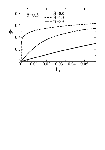
Figure 1: Staggered magnetization $\phi_{s}$ as a function of the staggered field $h_{s}$ for an isolated spin chain with bond alternation $\delta=0.5$. The solid, broken and dot-dashed lines are the magnetization curves for $\tilde{H}=0.0,1.5$ and $2.5$, respectively.

In Fig. 1, we summarize characteristic profiles of the staggered magnetization $\phi_{s}$ with $\tilde{H}$ being fixed. When $\tilde{H}=0$, the system has the triplet-excitation gap over the dimer-singlet ground state stabilized by the bond alternation $(\delta=0.5)$. In fact, the magnetization curve in staggered fields has a finite derivative at the origin, as seen from the solid line in Fig. 1, implying that the dimerized ground state is stable up to a certain critical value. The introduction of an external field decreases the spin gap, and eventually triggers the quantum phase transition to a gapless phase (so-called Tomonaga-Luttinger phase) at $\tilde{H}=1.5$, which is accompanied by the divergence of the spin susceptibility shown as the dashed line in Fig. 1. It is seen that the staggered susceptibility takes a finite value again in the large field region ($\tilde{H}=2.5$), implying that the spin gap phase with the magnetization plateau is stabilized, for which a finite interchain coupling is necessary to destroy the spin-gap state.

III Effects of the interchain coupling

We now discuss how the interchain coupling affects the magnetization process in the Q1D system, following the procedure outlined above. In the following we will explicitly use the bare external field $H$ instead of $\tilde{H}$ ($H=\tilde{H}+h_{u}$).

In Fig. 2, we show the magnetization curve calculated for the Q1D system, which is compared with that for the pure 1D case ($J^{\prime}=0$).

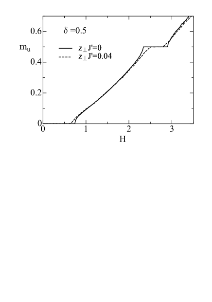
Figure 2: Magnetization curves for $\delta=0.5$ as a function of the applied field $H$. The solid and broken lines are the results calculated for an isolated chain ($z_{\perp}J^{\prime}=0$) and weakly coupled chains ($z_{\perp}J^{\prime}=0.04$), respectively.

Note that the ground-state for the 1D case is either in the singlet-dimer phase ($\delta>0.25$) or in the Haldane phase ($\delta<0.25$). We show the magnetization for the dimer-singlet phase ($\delta=0.5$) as an example, since that for the Haldane phase exhibits a similar behavior. Let us begin with the magnetization for the 1D case. Since the system is in the singlet-dimer phase with the spin excitation gap, the uniform magnetization does not appear up to the critical field $H_{c0}$. Beyond the critical field, the magnetization begins to increase and the system enters the Tomonaga-Luttinger liquid phase, which is immediately driven to a magnetically ordered phase upon introducing the interchain coupling. Further an increase in the field drives the system to another plateau state at $m_{u}=1/2$. This spin-gap phase with $m_{u}=1/2$ is expected to be stable against the introduction of the interchain coupling. However, it should be noticed that the spin-gap vanishes at both ends of the magnetization plateau, so that the width of the plateau should be considerably reduced by the interchain coupling. We can see that this is indeed the case for the results in Fig.2.

To see the above behavior in more detail, we show the phase diagram for the Q1D spin system with the interchain coupling $z_{\perp}J^{\prime}=0$ and $0.04$ in Fig. 3.

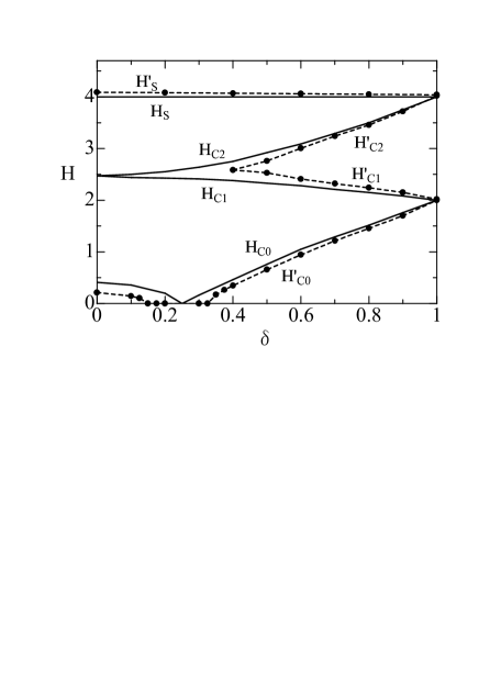
Figure 3: Phase diagram for the Q1D spin system. The solid and broken lines represent the phase diagram for an isolated chain ($z_{\perp}J^{\prime}=0$) and weakly coupled chains ($z_{\perp}J^{\prime}=0.04$), respectively. The uniform magnetization takes the quantized value at $m_{u}=0$ in the region from $0$ to $H_{c1}$ ($H^{\prime}_{c1}$), $m_{u}=1/2$ in the region from $H_{c2}$ ($H^{\prime}_{c2}$) to $H_{c3}$ ($H^{\prime}_{c3}$), and $m_{u}=1$ above $H_{s}$ ($H^{\prime}_{s}$). In other regions, the magnetization varies continuously.

Note that our phase diagram for the isolated chain ($z_{\perp}J^{\prime}=0$) agrees fairly well with that already obtained by the exact diagonalization method. Tone_1 Let us consider how the interchain coupling affects the plateau region with $m_{u}=1/2$, which is stabilized by the bond alternation. As seen from Fig. 3, the region of this phase is extended with increasing $\delta$. On the other hand, when the interchain coupling is introduced, the quantum fluctuation stabilizing the plateau is suppressed, and thus the region for the $m_{u}=1/2$ plateau is reduced.

We note here that the phase diagram obtained here is qualitatively valid except for an extreme case, $\delta\sim 1$, where the system is approximately described by an assembly of isolated dimers for $J^{\prime}=0$. When a finite interchain coupling $J^{\prime}$ is introduced for such almost isolated dimers, the system first forms the ladders rather than the chains for two-dimension. In this case, our approach based on the interchain mean-field theory may not be sensible. To treat the critical phenomena in this region, we need more precise treatment beyond mean-field theory, which is now under consideration.

Before closing this section, a brief comment is in order for the magnetization process in the Q1D Haldane system with a ferromagnetic interchain coupling, $J^{\prime}<0$. By rewriting the effective Hamiltonian, the critical points of the system with the ferromagnetic interchain couplings are given as,

$$H^{\prime}_{c0}(J^{\prime}=-|J^{\prime}|)=H^{\prime}_{c0}(J^{\prime}=|J^{\prime}|)$$ (9)

$$H^{\prime}_{c1,c2}(J^{\prime}=-|J^{\prime}|)=H^{\prime}_{c1,c2}(J^{\prime}=|J^{\prime}|)-z_{\perp}|J^{\prime}|$$ (10)

$$H^{\prime}_{s}(J^{\prime}=-|J^{\prime}|)=H^{\prime}_{s}(J^{\prime}=|J^{\prime}|)-2z_{\perp}|J^{\prime}|.$$ (11)

As easily seen from these formulae, the width of the plateau $H^{\prime}_{c2}-H^{\prime}_{c1}$ does not depend on the sign of $J^{\prime}$ in the framework of our mean-field treatment.

IV Effects of single-ion anisotropy

In this section, we discuss the effect of single-ion anisotropy with the Hamiltonian, ${\cal H}_{D}=D\sum_{i}(S^{\alpha}_{i})^{2}$. We consider two cases of anisotropy with respect to the direction of an applied magnetic field, i.e. $D\perp H$ ($\alpha=y$) and $D\parallel H$ ($\alpha=z$). By choosing the $x$-axis as the axis for the magnetic order, we discuss the magnetic properties of the Q1D system.

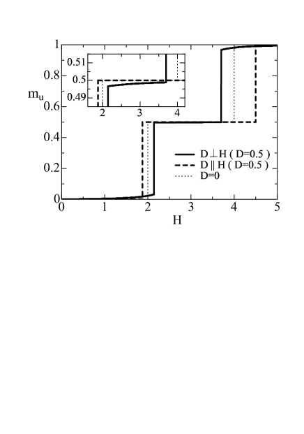
Figure 4: Magnetization curves for the isolated dimer system ($\delta=1$). For $D\parallel H(D=0.5)$, $D\perp H(D=0.5)$ and $D=0$. The inset shows the behavior around the plateau $m_{u}=1/2$.

To begin with, let us consider a simple system in the isolated-dimer limit with $(\delta,J^{\prime})=(1,0)$, which provides us with some insight into the role of single-ion anisotropy. The magnetization curves for $D=0.5$ are shown as the broken line ($D\parallel H$) and the solid line ($D\perp H$) in Fig.4. Note that the magnetization shows jumps in a magnetic field, reflecting the isolated dimer-singlet ground state When $D\parallel H$, the plateaus with $m_{u}=0$, $1/2$ and $1$ appear in the magnetization process clearly. On the other hand, in the case of $D\perp H$, the plateau is not exactly flat but is smeared by the Van Vleck contribution, as seen from the enlarged picture in the inset. This is because the total $S^{z}$ is not a conserved quantity for the case of $D\perp H$ even for $h_{s}=0$, which is in contrast to the case of $D\parallel H$. We also find that the width of the $m_{u}=1/2$ plateau is increased (decreased) upon introducing anisotropy, $D\parallel H$ ($D\perp H$). Therefore, the observation of the plateau structure may be somewhat difficult for $D\perp H$ in generic Q1D spin systems, because of shrinking of the width as well as smearing due to the Van Vleck term.

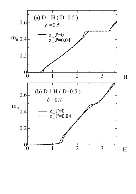
Figure 5: Magnetization curves for the Q1D system: (a) $D\parallel H(D=0.5)$ and $\delta=0.5$, and (b) $D\perp H(D=0.5)$ and $\delta=0.7$. The solid and broken lines show the results for $z_{\perp}J^{\prime}=0$ and $0.04$, respectively.

Keeping the above properties in mind, we now consider the magnetization process for the pure 1D as well as the Q1D systems. The numerical results are summarized in Fig. 5. Shown in Fig. 5(a) are the magnetization curves for $D\parallel H(D=0.5)$ and $\delta=0.5$, Since the presence of anisotropy, $D\parallel H$, has a tendency to stabilize the $m_{u}=1/2$ plateau, as mentioned above, thus increasing the plateau width compared with the isotropic case $D=0$ (see Fig. 2). It is also seen that the plateau state is rather stable against the introduction of the interchain coupling.

In Fig. 5 (b), we show the magnetization curves for the case of $D\perp H$ with bond alternation $\delta=0.7$. In contrast to the above $D\parallel H$ case, the plateau is indeed obscured both for the 1D (solid line) and Q1D systems (dashed line), which is due to the Van Vleck contribution. Therefore, in order to obtain the phase transition point correctly, it is necessary to consider another proper quantity characterizing the transition clearly. For this purpose, we evaluate the staggered magnetization in the $x$-axis. The calculated results for a single-chain system are plotted (broken line) together with the uniform magnetization (solid line) in Fig. 6. We note that a negligibly small staggered field $h_{s}=1.0\times 10^{-5}$ is added to stabilize the spontaneous staggered magnetization. It is seen that although the plateaus at $m_{u}=0,1/2$ and $1$ are vague, the phase transition point can be determined clearly at which the staggered magnetization vanishes. This is used to determine the phase diagram for the case of $D\perp H$.

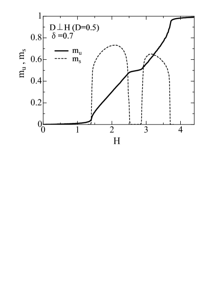
Figure 6: Uniform and staggered magnetizations for an isolated spin chain when $D\perp H$ ($D=0.5$).

Finally, we show the $\delta$-$H$ phase diagram for $D\parallel H$ and $D\perp H$ in Fig. 7 (a) and (b). In these figures, the solid and broken lines give the phase diagrams for an isolated 1D chain and weakly coupled chains, respectively. We note that when $J^{\prime}=H=0$, the quantum phase transition between the Haldane phase and the singlet-dimer phase occurs at the critical point $\delta_{c}\simeq 0.23$ for $D=0.5$. Tone_1 ; Hida_1 In the case of $D\parallel H$, the effects of the interchain couplings are analogous to those for the $D=0$ case (see Fig. 3). On the other hand, when the system has anisotropy in the $y$-direction, i.e. $D\perp H$, the phase diagram exhibits a quite different feature in contrast to the $D\parallel H$ case. In particular, the $m_{u}=1/2$ plateau region is reduced considerably both for the pure 1D as well as the Q1D systems.

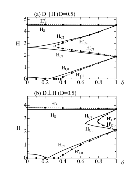
Figure 7: Phase diagrams for the Q1D quantum spin chain with single-ion anisotropy. The solid and broken lines are the phase boundaries for an isolated chain ($z_{\perp}J^{\prime}=0$) and weakly coupled chains ($z_{\perp}J^{\prime}=0.04$), respectively. The meanings of the critical fields and the corresponding phases are as in Fig. 3.

V Summary

We have studied the magnetization process for a Q1D $S=1$ antiferromagnet with bond alternation. By combining the density matrix renormalization group method with the interchain mean-field treatment, the magnetic properties have been discussed. It has been shown that the introduction of the interchain coupling enhances the antiferromagnetic correlation, thereby reducing the width of the plateau in the magnetization curve.

We have also discussed the effects of single-ion anisotropy, which sometimes plays an important role for understanding experimental findings in $S=1$ spin systems. It has been clarified that the magnetization curves exhibit distinct behaviors depending on the relative direction between single-ion anisotropy and an applied field. In particular, we have found that the magnetization plateau in the case of $D\perp H$ is rather unstable against the interchain coupling, and also suffers from the smearing effect due to the Van Vleck contribution, making the experimental observation somewhat difficult.

References

- (1) F. D. M. Haldane, Phys. Lett. 93A, 464 (1983); Phys. Rev. Lett. 50, 1153 (1983).
- (2) I. Affleck, T. Kennedy, E. H. Lieb, and H. Tasaki, Phys. Rev. Lett. 59, 799 (1987); Commun. Math. Phys. 115, 477 (1988).
- (3) I. Affleck, and F. D. M. Haldane, Phys. Rev. B 36, 5291 (1987).
- (4) R. R. P. Singh and M. P. Gelfand, Phys. Rev. Lett 61, 2133 (1988).
- (5) S. Yamamoto, Phys. Rev. B 52, 10 170 (1995).
- (6) C. Yasuda, S. Todo, M. Matsumoto, and H. Takayama, Phys. Rev. B 64, 092405 (2001); M. Matsumoto, C. Yasuda, S. Todo, and H. Takayama, Phys. Rev. B 65, 014407 (2002).
- (7) Y. J. Kim and R. J. Birgeneau, Phys. Rev. B 62, 6378 (2000).
- (8) A. Koga, and N. Kawakami, Phys. Rev. B 61, 6133 (2000).
- (9) Y. Kato, and A. Tanaka, J. Phys. Soc. Jpn. 63, 1277 (1994).
- (10) K. Totsuka, Y. Nishiyama, N. Hatano, and M. Suzuki, J. Phys.: Condens. Matter 7, 4895 (1995).
- (11) T. Tonegawa, T. Nakao, and M. Kaburagi, J. Phys. Soc. Jpn. 65, 3317 (1996).
- (12) W. Chen, K. Hida and B. C. Sanctuary, J. Phys. Soc. Jpn. 69, 237 (2000).
- (13) T. Sakai, and M. Takahashi, Phys. Rev. B. 42, 4537 (1990).
- (14) T. Sakai, Phys. Rev. B. 62, R9240 (2000).
- (15) T. Sakai, and M. Takahashi, J. Phys. Soc. Jpn. 62, 750 (1993).
- (16) T. Hikihara: preprint (cond-mat/0006445). A. Kolezhuk, Phys. Rev. B. 62, R6057 (2000).
- (17) W. J. L. Buyers, P. M. Morra, R. L. Armstrong, M. J. Hogan, P. Gelrach, and K. Hiraawa, Rhys. Rev. Lett. 56, 3371 (1986); M. Steiner, K. Kakurai, J. K. Kjems, D. Petitgrand, and R. Pynn, J. Appl. Phys. 61, 3953 (1987).
- (18) J. P. Renard, M. Verdaguer, L. P. Regnault, W. A. C. Erkelens, J. Rossat-Migdot, and W. G. Stirling, Europhys. Lett. 3, 945 (1987).
- (19) Y. Uchiyama, Y. Sasago, I. Tsukada, K. Uchinokura, A. Zheludev, T. Hayashi, N. Miura, and P. Böni, Rhys. Rev. Lett. 83, 632 (1999); A. Zheludev, T. Masuda, I. Tsukada, Y. Uchiyama, K. Uchinokura, P. Böni, and S.-H. Lee, Phys. Rev. B. 62, 8921 (2000); A. Zheludev, T. Masuda, K. Uchinokura, and S. E. Nagler, Phys. Rev. B. 64, 134415 (2001).
- (20) Z. Honda, K. Katsumata, H. Aruga Katori, K. Yamada, T. Ohishi, T. Manabe, and M. Yamashita, J. Phys. Condens. Matter 9, 3487 (1997).
- (21) Z. Honda, H. Asakawa, and K. Katsumata, Phys. Rev. Lett. 81, 2566 (1998); Z. Honda, K. Katsumata, Y. Nishiyama and I. Harada, Phys. Rev. B. 63, 064420 (2001).
- (22) M. Hagiwara, Y. Narumi, K. Kindo, M. Kohno, H. Nakano, R. Sato, and M. Takahashi, Phys. Rev. Lett. 80, 1312 (1998).
- (23) A. Escuer, R. Vincente, and X. Solans, J. Chem.Soc. Dalton Trans. 531 (1997); Y. Narumi, M. Hagiwara, M. Kohno, and K. Kindo, Phys. Rev. Lett. 86, 324 (2001).
- (24) Y. Narumi, M. Hagiwara, and K. Kindo: preprint.
- (25) S. R. White, Phys. Rev. Lett. 69, 2863 (1992); Phys. Rev. B. 48, 10345 (1993).
- (26) T. Nishino and K. Okunishi, J. Phys. Soc. Jpn. 64, 4084 (1995); Y. Hieida, K. Okunishi and Y. Akutsu, Phys. Lett. A. 233, 464 (1997); Y. Hieida, K. Okunishi, and Y. Akutsu, Phys. Rev. B. 64, 224422 (2001).
- (27) H. J. Schulz, Phys. Rev. Lett. 77, 2790 (1996); Z. Wang, Phys. Rev. Lett. 78, 126 (1997); A. W. Sandvik, Phys. Rev. Lett. 83, 3069 (1999); S. Wessel and S. Haas, Eur. Phys. J. B. 16, 393 (2000).