Anomalous relaxation kinetics of biological lattice-ligand binding models

Abstract

We discuss theoretical models for the cooperative binding dynamics of ligands to substrates, such as dimeric motor proteins to microtubules or more extended macromolecules like tropomyosin to actin filaments. We study the effects of steric constraints, size of ligands, binding rates and interaction between neighboring proteins on the binding dynamics and binding stoichiometry. Starting from an empty lattice the binding dynamics goes, quite generally, through several stages. The first stage represents fast initial binding closely resembling the physics of random sequential adsorption processes. Typically this initial process leaves the system in a metastable locked state with many small gaps between blocks of bound molecules. In a second stage the gaps annihilate slowly as the ligands detach and reattach. This results in an algebraic decay of the gap concentration and interesting scaling behavior. Upon identifying the gaps with particles we show that the dynamics in this regime can be explained by mapping it onto various reaction-diffusion models. The final approach to equilibrium shows some interesting dynamic scaling properties. We also discuss the effect of cooperativity on the equilibrium stoichiometry, and their consequences for the interpretation of biochemical and image reconstruction results.

I Introduction

How does a system evolve towards its steady state? Sometimes the answer is quite simple and the relaxation process is merely an exponential decay. If the deviations from equilibrium are small Onsager’s regression hypothesis onsager31 asserts that the relaxation is governed by the same laws as the fluctuations in equilibrium. This hypothesis certainly fails for systems with an absorbing steady state such as simple models for diffusion-limited chemical reactions torney83 ; toussaint83 ; racz85 ; peliti86 ; nielaba92 . Here there are no fluctuations in the steady state but the approach towards the absorbing state is critical in the sense that it exhibits slow power-law decay and universal scaling behavior cardyreview . Most of these models are chosen to be mathematically transparent hoping that they still resemble some of the essential features of actual systems occurring in nature. Unfortunately, experimentally accessible systems where the above theoretical ideas can be tested explicitly have remained rare to date.

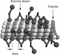
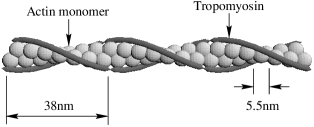
a)	b)

Figure 1: a) Kinesin dimers can bind one head or both heads to a one-dimensional lattice (tubulin protofilament). Binding sites are located on $\beta$-tubulin subunits (dark) while $\alpha$-subunits (bright) are irrelevant for our study. b) Tropomyosin binds to an actin filament by occupying $7$ lattice sites. There is a strong attractive interaction between the ends of bound tropomyosin molecules.
b) © 2001, Biophysical Society vilfan2001c

In this contribution we discuss the kinetics of some macromolecular assembly processes relevant for the formation of functional structures in cells. In particular, we are interested in the dynamics of ligand-substrate binding, where the substrate is a one- or two-dimensional lattice and the ligands are dimers or oligomers. Examples for such systems are illustrated in Fig. 1. Binding of dimeric myosin to actin filaments conibear98 can behave in a similar way as dimeric kinesin on microtubules. Similar interactions of large supramolecular biological polymers with protein ligands such as DNA with proteins or viruses with antibodies are also a quite intensive area of research. As will become clear in later chapters the kinetics of these systems shows interesting anomalous dynamics which is closely related to the mathematical models of simple diffusion-reaction systems discussed above.

Fig. 1a shows a schematic representation of a “decoration experiment” where dimeric motor enzymes (ligands) are deposited on their corresponding molecular track (substrate) mandelkow_hoenger99 ; hoenger00 . For kinesin motors, these tracks are microtubules, hollow cylinders usually consisting of $13$ protofilaments, linear polymers composed of alternating $\alpha$- and $\beta$-tubulin subunits. The kinesin binding sites are located on the $\beta$ subunits (dark spheres) which form a helical (wound-up rhombic) lattice with a longitudinal periodicity of $8\,{\rm nm}$. Kinesin is a mechanochemical enzyme, which transforms (through an isothermal stochastic process) the chemical energy obtained from the hydrolysis of adenosine triphosphate (ATP) into motion along microtubules. Roughly speaking, kinesin has the following building plan: two globular heads (also called motor domains) with the functionality of ”legs” are joined together by a coiled-coil region into a tail which can bind to some cargo. The typical size of these proteins is in the range of several tens of nanometers.

Decoration techniques are usually performed in the absence of ATP hydrolysis. Then the motor enzymes are “passive” ligands which bind and unbind from their tubulin binding sites but do not actively move along microtubules. These systems have traditionally been used in biophysical chemistry to investigate the structure and the binding properties of kinesin mandelkow_hoenger99 ; hoenger00 , i.e. after waiting for the system to equilibrate the binding stoichiometry is measured and the structure is determined by cryo-electron microscopy followed by 3D image reconstruction. These investigations are key elements in understanding the binding patterns of kinesin motor domains under changing nucleotide conditions to get a complete picture on the different conformational states, which are involved in the kinesin walking mechanism schief2001 .

In the following sections we present a theoretical analysis of dimer adsorption-desorption kinetics with competing single and double bound dimers. Such analysis is extremely important for a quantitative analysis of decoration data vilfan2001a ; a theoretical analysis gives the binding stoichiometry in the equilibrium state in terms of binding constants for the first and second head of the dimer molecule. The dynamics of the approach to equilibrium is useful to estimate when an experimental system can be considered as equilibrated. Even more importantly, time-resolved decoration experiments (e.g. by using motor enzymes labelled by some fluorescent marker) combined with our theoretical analysis could provide new information about reaction rates which are to date not known completely. Understanding the kinetics of passive motors is undoubtedly a necessary prerequisite for studying the more complicated case of active motors at high densities capello_preprint . The model is also interesting in its own right since it contains some novel features of non-equilibrium dynamics of dimer adsorption-desorption models.

Fig. 1b shows a schematic representation of tropomyosin binding to an actin filament vilfan2001c . Actin filaments are one of the major compontents of the cytoskeleton. Like microtubules, they contribute to the mechanical stability of the cell and serve as tracks for molecular motors from the myosin family. This function is especially pronounced in muscle cells where both actin and myosin form filaments that can slide between each other and thereby cause the muscle to contract. Tropomyosin plays the key role in the control of skeletal muscle contraction. It binds to actin along its binding sites for myosin motors. When calcium ions are released as a response to a nerve signal, they cause tropomyosin to shift laterally thereby clearing the binding sites and allowing myosin to bind and produce force. Tropomyosin binding to action has several features which make it an interesting model system of statistical physics; each molecule covers seven actin monomers and interacts strongly with other tropomyosin molecules. As a consequence gaps between bound molecules can take a long time to heal. Although the gap dynamics has not yet been measured experimentally, the amount of data gathered in other kinetic studies provides plenty of information on the model parameters and allows to make quantitative predictions about the relaxation time. As it turns out vilfan2001c , these relaxation times can be as large as hours, which is short enough compared to the lifetime of actin filaments in a muscle cell, but essential when planning experiments with actin and tropomyosin assembled in vitro, especially when studying the myosin regulation fraser95 .

The outline of this article is as follows. In Section II we define the model for decoration of microtubules with dimeric motors which can bind either with one or with two heads as first introduced in Ref. vilfan2001a . In Section III we determine analytically the equilibrium state of this model. We study the dynamics of the model in Section IV, which extends the results presented in Ref. vilfan2001b . Section V studies the dynamics of the two-dimensional model with interactions and Section VI the dynamics of the one-dimensional $k$-mer model, which is a more generalized version of the results described in Ref. vilfan2001c . In the final section we give a summary and an outlook on future challenges in the field.

II Definition of the microtubule decoration model

Our model describes the experimental situation as found in most decoration assays. It starts with an empty tubulin sheet surrounded by a solution of double-headed kinesin molecules. The kinesin dimers can either attach with one or two heads onto binding sites located on $\beta$-tubulin. There seems to be convincing evidence that kinesin heads can bind on two adjacent binding sites only in longitudinal but not in lateral direction mandelkow_hoenger99 ; hoenger00 . This introduces a strong uniaxial anisotropy and distinguishes the adsorption process of protein dimers from simple inorganic dimers. The attached heads can also detach at some rate. A schematic representation of the decoration process onto tubulin sheets is given in Fig. 2.

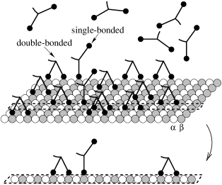
Figure 2: Schematic representation of the binding of kinesin dimers to a tubulin sheet. The binding sites are located on the $\beta$-tubulin subunits marked as grey balls. A dimer can attach either with one head to one binding site or with two heads on two adjacent sites along the same protofilament. Each binding site can be occupied by at most one kinesin head. Neglecting interactions between kinesin molecules results in a one-dimensional model with dimers decorating individual protofilaments.

To begin with, let us take into account only steric (hard-core) interactions and for now neglect nearest neighbour attractive interactions. Then we are left with a one-dimensional problem of kinesin dimers decorating a single protofilament (one-dimensional lattice) as shown in Fig. 2 and defined as follows. Kinesin is considered as a dimeric structure with its two heads tethered together by some flexible joint. Hence each dimer (kinesin protein) can bind one of its two heads (motor domains) to an empty lattice site vilfan2001a . The binding rate $k_{+1}\,c$ for this process is proportional to the solution concentration $c$ of the dimeric proteins. Successively, the dimer may either dissociate from the protofilament with a rate $k_{-1}$ or also bind its second head to an unoccupied site in front (f) of or behind (b) the already bound head (with front we always refer to the direction pointing towards the “+” end of the microtubule, which is the direction of motion for most motors from the kinesin family). Since kinesin heads and microtubules are both asymmetric structures the corresponding binding rates $k_{+2}^{f}$ and $k_{+2}^{b}$ are in general different from each other. The reverse process of detaching a front or rear head occurs at rates $k_{-2}^{f}$ and $k_{-2}^{b}$. A reaction scheme with all possible processes and their corresponding rate constants is shown in Fig. 3.

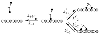
Figure 3: Reaction scheme for all binding and unbinding processes. The rates for binding and unbinding of the first head are given by $k_{+1}\,c$ and $k_{-1}$, respectively. The second head may bind to an unoccupied site in front (f) of or behind (b) the already bound head with rates $k_{+2}^{f}$ and $k_{+2}^{b}$. The corresponding reverse process of detaching a front or rear head occurs at rates $k_{-2}^{f}$ and $k_{-2}^{b}$.
© 2001, Academic Press vilfan2001a

In typical decoration experiments there is no external energy source, i.e. no ATP hydrolysis. Then the binding rates are not all independent of each other, but detailed balance dictates that the ratio of on- and off-rates has to equal the equilibrium binding constants

$$K_{1}=\frac{k_{+1}}{k_{-1}}\,,\quad\text{and}\quad K_{2}=\frac{k_{+2}^{b}}{k_{-2}^{b}}=\frac{k_{+2}^{f}}{k_{-2}^{f}}\,.$$ (1)

A particular coverage of the lattice is described as a sequence of dimers bound with both heads ($D$), one head only ($1$) and empty sites ($0$) (see Fig. 4). We denote the probabilities to find a certain lattice site in one of these states by $2n_{D}$, $n_{1}$ and $n_{0}$, respectively. Of course, normalization of the probabilities requires $n_{0}+n_{1}+2n_{D}=1$.

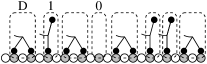
Figure 4: A configuration of bound kinesin molecules on a protofilament. The element $D$ represents a dimer with two bound heads, the element $1$ a dimer bound on one head and the element $0$ an empty lattice site (vacancy).
© 2001, Academic Press vilfan2001a

II.1 Particle-hole symmetry

Important information about the steady state and the dynamics of the system can be gained already by exploiting the symmetries of the kinetic process. Fig. 5 reveals a “particle-hole” symmetry by showing a transformation that maps the system onto one with the same reaction scheme, albeit with transformed kinetic constants. The details of the transformation are listed in Table 1.

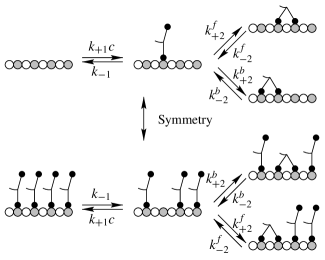
Figure 5: The one-dimensional dimer decoration model is invariant upon exchanging empty lattice sites $(0)$ with single-bonded dimers $(1)$ and the reaction rates according to $(k_{+1}c,k_{2\pm}^{f})\leftrightarrow(k_{-1},k_{2\pm}^{b})$.

The “particle-hole” exchange operation replaces dimers bound on a single head (“particles”) by vacant sites (“holes”) and vice versa. Dimers bound with both heads are kept invariant under the transformation. To obtain a system with an equivalent reaction scheme the transition rates have to be transformed as well. This is achieved by exchanging the attachment and detachment rate of the first head, $k_{+1}c\leftrightarrow k_{-1}$, and simultaneously switching the forward and backward binding rates of the second head, $k_{2\pm}^{f}\leftrightarrow k_{2\pm}^{b}$. As a consequence of this symmetry operations the equilibrium constant $K_{1}c$ is replaced by its reciprocal value while the binding constant of the second head $K_{2}$ is left unchanged.

Table 1: The dynamics of the one-dimensional dimer decoration model is invariant under the following “particle-hole” transformation.

	state			kinetic constants						equilibrium constants
Original	0	1	D	$k_{+1}c$	$k_{-1}$	$k_{+2}^{f}$	$k_{+2}^{b}$	$k_{-2}^{f}$	$k_{-2}^{b}$	$K_{1}c$	$K_{2}$
Transformed	1	0	D	$k_{-1}$	$k_{+1}c$	$k_{+2}^{b}$	$k_{+2}^{f}$	$k_{-2}^{b}$	$k_{-2}^{f}$	$1/(K_{1}c)$	$K_{2}$

This symmetry has immediate consequences on the equilibrium stoichiometry. Since the coverage in the steady state is solely a function of the quantities $K_{1}c$ and $K_{2}$ this symmetry implies that the mean number of dimers attached with both heads (which are mapped onto themselves) $n_{D}(K_{1}c,K_{2})$ is invariant upon interchanging the attachment and detachment rates of the first head,

$$n_{D}(1/K_{1}c,K_{2})=n_{D}(K_{1}c,K_{2})$$ (2)

Similarly the mean total number of bound heads per lattice site (binding stoichiometry), $\nu=2(n_{1}+n_{D})$, obeys the symmetry relation

$$\nu(1/K_{1}c,K_{2})=2-\nu(K_{1}c,K_{2})\;.$$ (3)

The symmetries can be best seen in a logarithmic-linear plot as shown in Fig. 6. From these relations we already conclude that the stoichiometry of dimers bound with both heads $n_{D}$ reaches its maximum at $K_{1}c=1$ and that the total stoichiometry is $\nu=1$ at that point.

II.2 Experimental parameter values

The kinetic constants for the binding of kinesin on microtubules have been determined by several groups hackney94 ; ma95 ; moyer98 ; mandelkow98 . The binding constants for the first head in the presence of ATP and low ionic strength have the values moyer98 $k_{+1}=20\,\mu{\rm M}^{-1}{\rm s}^{-1}$ and $k_{-1}=25\,{\rm s}^{-1}$, leading to $K_{1}=0.8\,\mu{\rm M}^{-1}$. $k_{-1}$ is much smaller in the presence of AMP-PNP or in the absence of a nucleotide, about $0.01\,{\rm s}^{-1}$ hancock99 . The binding constant $K_{2}$ can be estimated indirectly as the ratio between the detachment rate of the monomeric and the dimeric kinesin and has values between 2.7 (in the presence of ATP) and 20 (without a nucleotide) hancock99 . These values show that the model parameters depend strongly on the chemical conditions and the type of motor protein used in the experiment. A theoretical investigation allows for a systematic analysis and detailed classification of all the different regimes of binding kinetics in such a broad range of parameter values.

III Equilibrium stoichiometry

In this section we review results obtained for the equilibrium stoichiometry of the dimer binding model vilfan2001a . In this section we will discuss the one-dimensional model where some short-range interaction between the dimers is taken into account; two-dimensional models are studied in Sec. V.

III.1 Analytical solution for the binding stoichiometry

For the one-dimensional model the value of the mean occupation numbers in the steady state can quite easily be determined upon using detailed balance and the fact that the dimers have only a hard-core interaction. Because we have non-interacting dimers the probability to find a certain sequence of $0$’s, $1$’s and $D$’s (e.g. “0,1,D,D,1,D”, see Fig. 4) has to be invariant against permutations of these states. In such a random sequence the probability $p_{i}$ to find a particular state $0$, $1$ or $D$ at a certain site $i$ is given by

$$p_{i}=\frac{n_{i}}{n_{0}+n_{1}+n_{D}}\,.$$ (4)

Detailed balance requires that for each pair of possible configurations, their respective probabilities are in the same ratio as the transition rates between them. Hence the ratio of probabilities to find a sequence with a $1$ or $0$ at a certain place is

$$\frac{p_{1}}{p_{0}}=\frac{k_{+1}c}{k_{-1}}=K_{1}c\,.$$ (5)

Similarly, we get for transitions between $D$ and $01$:

$$\frac{p_{D}}{p_{0}p_{1}}=\frac{k_{+2}^{f}}{k_{-2}^{f}}=\frac{k_{+2}^{b}}{k_{-2}^{b}}=K_{2}\,.$$ (6)

These two equations, together with the normalization condition, uniquely determine the values $n_{0}$, $n_{1}$ and $n_{D}$. The number of dimers bound with both heads is given by

$$n_{D}=\frac{1}{2}-\frac{1}{2}\left(\frac{4K_{1}K_{2}c}{(1+K_{1}c)^{2}}+1\right)^{-\frac{1}{2}}$$ (7)

and the number of dimers bound with one head

$$n_{1}=\frac{K_{1}c}{K_{1}c+1}\left(\frac{4K_{1}K_{2}c}{(1+K_{1}c)^{2}}+1\right)^{-\frac{1}{2}}$$ (8)

The stoichiometry, i.e. the total number of heads per binding site $\nu=2(n_{1}+n_{D})$ then reads

$$\nu=1+\frac{K_{1}c-1}{K_{1}c+1}\left(\frac{4K_{1}K_{2}c}{(1+K_{1}c)^{2}}+1\right)^{-\frac{1}{2}}\;.$$ (9)

The number of dimers bound with both heads per lattice site reaches its maximum $n_{D}^{\rm max}=(1-1/\sqrt{K_{2}+1})/2$ for $K_{1}c=1$. For an illustration of all these equations see Fig. 6.

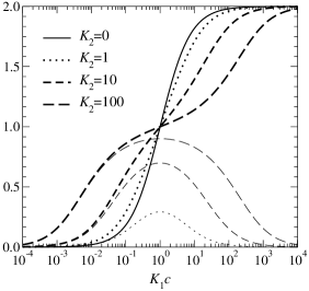
Figure 6: Binding stoichiometry $\nu$ as a function of the solution concentration $c$ and the constant $K_{2}$. The thick curves show the total number of heads per lattice site $\nu$ (9). The thin curves show the fraction of binding sites occupied with double-attached dimers $2n_{D}$ (7).

III.2 Alternative derivation of the binding stoichiometry

Here we present an alternative derivation of the binding stoichiometry which has the additional benefit that it can also be used for two-dimensional lattices where dimers can bind in either direction. The idea is to relate the equilibrium stoichiometry of the flexible dimer model to that of a stiff dimer model – a model where dimers can only bind as whole. Once we have specified the mapping one can determine the stoichiometry of the general model from the stoichiometry of the stiff dimer model in one dimension which has been known for quite a long time hill57 already and represents a special case of the solution by McGhee and von Hippel mcghee74

$$n=\frac{1}{2}\left(1-\frac{1}{\sqrt{4K+1}}\right)\;.$$ (10)

Note, that in this notation the binding constant $K$ contains the concentration $c$. In equilibrium, a mapping between the stiff and flexible dimer model is possible because of detailed balance and because transitions between states $0$ and $1$ are uncorrelated with the surrounding configuration. Let’s denote the equilibrium binding constant, the dimer and vacancy density in the stiff dimer model by $K$, $\bar{n}_{D}$ and $\bar{n}_{0}$, respectively. Then, detailed balance gives the following relation between these densities and the equilibrium binding constant, $K=\bar{n}_{D}/\bar{n}_{0}^{2}$. In the same way detailed balance implies $K_{2}=n_{D}/(n_{0}n_{1})$ and $K_{1}c=n_{1}/n_{0}$ for the general dimer model. The absence of correlations allows us to group together the states $1$ and $0$ of the general model into a single state which we identify with the vacant state $\bar{0}$ of the stiff dimer model. This gives the mapping as summarized in Table 2.

Table 2: Mapping between the equilibrium states of the stiff and the flexible dimer model.

	Stiff	Flexible
Densities	$\bar{n}_{D}$,   $\bar{n}_{0}$	$n_{D}$,   $n_{0}+n_{1}$
Binding constants	$K$	$K_{1}c$, $K_{2}$
Equilibrium condition	$K=\frac{\bar{n}_{D}}{\bar{n}_{0}^{2}}$	$K_{1}c=\frac{n_{1}}{n_{0}}$, $K_{2}=\frac{n_{D}}{n_{0}n_{1}}$

From this table we can infer that the number of fully bound dimers per lattice site in the flexible dimer model is given as

$$n_{D}(K_{1}c,K_{2})=\bar{n}_{D}(K)=\bar{n}_{D}\left(\frac{K_{2}K_{1}c}{(1+K_{1}c)^{2}}\right)\;,$$ (11)

and the number of dimers bound with one head as

$$n_{1}(K_{1}c,K_{2})=\frac{K_{1}c}{1+K_{1}c}\bar{n}_{0}(K)=\\ =\frac{K_{1}c}{1+K_{1}c}\left(1-\frac{1}{2}\bar{n}_{D}\left(\frac{K_{2}K_{1}c}{(1+K_{1}c)^{2}}\right)\right)\;.$$ (12)

In the one-dimensional case we can insert Eq. (10) and reproduce Eqs. (7) and (8). Note that the mapping reduces the number of parameters by one leading to a quite significant simplification. Though the stiff dimer model has not yet been solved analytically in two dimensions, the model with a single parameter can easily be solved by Monte-Carlo simulation (e.g., phares93b ). The entropy of a two-dimensional lattice fully covered with dimers is even known exactly kasteleyn61 ; temperley61 .

IV Dynamics

In this section we will learn that the relaxation towards the equilibrium state described in the previous section is by no means a simple process characterized by a single time scale but actually shows quite interesting anomalous kinetics. We find different scenarios depending on the value of the equilibrium binding constants $K_{2}$ of the second head. If $K_{2}\lesssim 1$ there are comparatively few double-bonded dimers in the steady state. Consequently cooperative effects and correlations are less important implying that the equilibration process is exponential with the time scale given by the rates $k_{+1}c$ and $k_{-1}$. The dynamics changes drastically if the second head is very likely to bind, $K_{2}\gg 1$. Then, the equilibrium state will consist mainly of dimers bound with both heads aligned with twice the period of the lattice. Their positions are correlated at a length scale given by the average distance between defects in the periodic pattern (either vacancies or single-bonded dimers). As we will detail in this section these correlations lead to a dynamics which is slowed down drastically as compared to the kinetics of individual dimers.

In the following we will mainly concentrate on the case $K_{1}c\ll 1$, to which we refer as the “stiff dimer model”, reflecting the fact that dimers are only likely to be found in the state with both heads bound. In this limit we can discuss the essential features of our model, which include the anomalous relaxation kinetics. Because of the particle-hole symmetry (Sect. II.1) which transforms $K_{1}c\to 1/(K_{1}c)$, the results apply equally well for $K_{1}c\gg 1$. The other interesting limiting case is the situation with $K_{2}\gg 1$ and $K_{1}c\approx 1$. In this limit the dynamics is essentially similar to the case $K_{1}c\ll 1$, but more complicated in detail because we have to consider all three states, i.e. empty sites, dimers bound with one head and dimers bound with both heads.

IV.1 The stiff dimer limit

It turns out that most interesting features of the model can already be discussed if we restrict ourselves to the limit

$$K_{2}\gg 1,\qquad K_{1}c\ll 1$$ (13)

with $K=K_{1}K_{2}c$ fixed at a value which allows the equilibrium state to consist mainly of dimers bound with both heads. The first condition of Eq. (13) states that the second head is unlikely to be found in the unbound state if it has a place where it can bind. The second condition implies that isolated single-site vacancies are unlikely to be occupied with single-bonded dimers. Therefore, our model reduces to a dimer deposition-evaporation model where the dimers can only bind and unbind with both heads at the same time. We will refer to this model as “stiff dimer model” in the following. The vacancy concentration $n_{0}$ in the steady state, given as $1-n_{1}-2n_{D}$ in Eq. (7) and (8) then simplifies to

$$n_{0}=1/\sqrt{1+4K}\;.$$ (14)

The stiff dimer model describes dimers that bind at once to a pair of empty lattice sites and is characterized by the effective attachment rate of a whole dimer to an empty pair of sites, $k_{+}c$, an effective detachment rate $k_{-}$, and a rate with which a dimer can move diffusively without detaching, $r_{d}$. Depending on whether the diffusion or the detachment rate is larger, we will distinguish between the diffusive and the non-diffusive case. The stiff dimer model is similar to conventional dimer deposition models privman92 , however with the difference that the attachment and detachment constants $k_{+}$ and $k_{-}$ also depend on whether the neighboring sites are occupied or not (but we will show that this dependence becomes irrelevant in the non-diffusive case).

IV.1.1 Mapping between the general model and the stiff dimer model

In the following we describe how the kinetics of the stiff dimer model follows from our general dimer model. In the limit we are considering, the detachment of a single-bound dimer is always much faster than the attachment of a new one ($k_{-1}\gg k_{+1}c$, following from $K_{1}c\ll 1$) and the attachment of the second head much faster than its detachment ($k_{+2}^{f,b}\gg k_{-2}^{f,b}$, following from $K_{2}\gg 1$). We do not put any other limitations on the reaction rates for now.

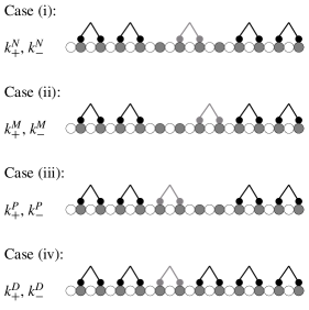
Figure 7: Four cases for the binding of a new dimer (grey) in a gap between already bound ones (black). The effective binding rates are $k_{+}^{N,M,P,D}$ and the unbinding rates $k_{-}^{N,M,P,D}$.

In a general treatment, the attachment and detachment rates also depend on the occupancy of the neighboring sites. We therefore have to distinguish between four cases: both neighbors empty, front neighbor occupied, rear neighbor occupied and both neighbors occupied.

• Case (i): Both neighbors empty. A dimer attaches with its first head at the rate $k_{+1}c$. Afterwards, the second head can attach at the total rate $k_{+2}^{f}+k_{+2}^{b}$, while the first head can detach with rate $k_{-1}$. This leads to the total attachment rate per lattice site

  $$k^{N}_{+}c=\frac{k_{+1}c(k_{+2}^{f}+k_{+2}^{b})}{k_{-1}+k_{+2}^{f}+k_{+2}^{b}}\;.$$ (15)

  The process of detachment starts with the detachment of the front or rear head. The detachment gets completed if the other head detaches too (rate $k_{-1}$) and fails if the detached head reattaches again (rate $k_{+2}^{f}+k_{+2}^{b}$). The detachment rate then becomes

  $$k^{N}_{-}=\frac{k_{-1}(k_{-2}^{f}+k_{-2}^{b})}{k_{-1}+k_{+2}^{f}+k_{+2}^{b}}\;.$$ (16)

• Case (ii): Front neighbor occupied. There are two pathways that lead to binding next to an occupied site. The first head can either attach on the site next to the occupied one or one site further away, both at the rate $k_{+1}c$. In the first case the probability that the second head will attach before the first one detaches is $k_{+2}^{b}/(k_{-1}+k_{+2}^{b})$. In the second case the probability that the second head attaches in front of the first one is $k_{+2}^{f}/(k_{-1}+k_{+2}^{f}+k_{+2}^{b})$. These two terms taken together give the attachment rate to the given pair of sites

  $$k^{M}_{+}c=k_{+1}c\left(\frac{k_{+2}^{b}}{k_{-1}+k_{+2}^{b}}+\frac{k_{+2}^{f}}{k_{-1}+k_{+2}^{f}+k_{+2}^{b}}\right)\;.$$ (17)

  If the process of detachment starts with detaching the front head (rate $k_{-2}^{f}$), the probability that the whole dimer will detach afterwards is $k_{-1}/(k_{-1}+k_{+2}^{f}+k_{+2}^{b})$. If it starts with detaching the rear head (rate $k_{-2}^{b}$), this probability is $k_{-1}/(k_{-1}+k_{+2}^{b})$. This gives the total detachment rate

  $$k^{M}_{-}=k_{-1}\left(\frac{k_{-2}^{b}}{k_{-1}+k_{+2}^{b}}+\frac{k_{-2}^{f}}{k_{-1}+k_{+2}^{f}+k_{+2}^{b}}\right)\;.$$ (18)

• Case (iii): Rear neighbor occupied. This case is analogous to the previous one, except that the indices $f$ and $b$ have to be interchanged. The attachment rate becomes

  $$k^{P}_{+}c=k_{+1}c\left(\frac{k_{+2}^{b}}{k_{-1}+k_{+2}^{f}+k_{+2}^{b}}+\frac{k_{+2}^{f}}{k_{-1}+k_{+2}^{f}}\right)$$ (19)

  and the detachment rate

  $$k^{P}_{-}=k_{-1}\left(\frac{k_{-2}^{b}}{k_{-1}+k_{+2}^{f}+k_{+2}^{b}}+\frac{k_{-2}^{f}}{k_{-1}+k_{+2}^{f}}\right)\;.$$ (20)

• Case (iv): Both neighbors occupied. In this case the dimer binds into a gap of exactly two sites. If the first head attaches to the front site in the gap (rate $k_{+1}c$), the probability for the second one to attach before the first one detaches is $k_{+2}^{b}/(k_{-1}+k_{+2}^{b})$. Together with the analogous case in which the first head attaches to the rear site inside the vacancy, the total attachment rate becomes

  $$k^{D}_{+}c=k_{+1}c\left(\frac{k_{+2}^{b}}{k_{-1}+k_{+2}^{b}}+\frac{k_{+2}^{f}}{k_{-1}+k_{+2}^{f}}\right)\;.$$ (21)

  After the front head has detached (rate $k_{-2}^{f}$), the probability that the whole dimer will follow is $k_{-1}/(k_{-1}+k_{+2}^{f})$. Adding the pathway starting with the detachment of the rear head gives the detachment rate

  $$k^{D}_{-}=k_{-1}\left(\frac{k_{-2}^{b}}{k_{-1}+k_{+2}^{b}}+\frac{k_{-2}^{f}}{k_{-1}+k_{+2}^{f}}\right)\;.$$ (22)

Of course, all these rates obey detailed balance, which states that

$$\frac{k_{+}c}{k_{-}}=K=K_{1}K_{2}c\;.$$ (23)

Processes in which one head detaches on one side and subsequently attaches on the other side also lead to an explicit diffusion of attached dimers. A diffusive step forwards occurs if the rear head detaches (rate $k_{-2}^{b}$) and reattaches on the front side (probability $k_{+2}^{f}/(k_{-1}+k_{+2}^{f}+k_{+2}^{b})$). The hopping rate (which is, of course, equal for backward steps) then reads

$$r_{d}=\frac{k_{+2}^{f}k_{+2}^{b}}{K_{2}(k_{-1}+k_{+2}^{f}+k_{+2}^{b})}\;.$$ (24)

So far we have shown that in the limit $K_{2}\gg 1$ our model can be mapped onto a simple dimer model. But, depending on parameters, this can happen in two qualitatively different ways. First, if the detachment rate is smaller than the diffusion rate $k_{-}\ll r_{d}$, which is equivalent to the condition

$$k_{-1}\ll\frac{1}{\frac{1}{k_{+2}^{f}}+\frac{1}{k_{+2}^{b}}}\;,$$ (25)

we get the diffusive limit. In the opposite limit, a dimer is unlikely to make a diffusive step before it detaches and we call that the non-diffusive limit. In the non-diffusive limit, the effective dimer attachment ($k_{+}c$) and detachment ($k_{-}$) rates become equal in all four cases, i.e. they become independent of the surroundings of a dimer.

To summarize, the stiff dimer model in the non-diffusive limit, to which we will concentrate in the following, describes dimers that can bind to any free pair of lattice sites with equal rate, namely $k_{+}c$ and can detach with a rate $k_{-}$. The dimer cannot move along the lattice and it always stays joined (cannot regroup its two parts with parts of other dimers). Although dimers cannot diffuse directly, in the case of high lattice coverage we can still introduce an effective diffusion which describes dimers near a gap detaching and reattaching on the other side of the gap. This simplified model still captures all the essential aspects of the non-equilibrium dynamics.

IV.1.2 Related dimer models

Similar dimer adsorption models have been studied previously privman92 ; barma93 ; stinchcombe93 ; eisenberg97 . Privman and Nielaba privman92 studied the effect of diffusion on the dimer deposition process (neglecting dimer desorption). There are several key differences to our model, the most important of which is that diffusion without detachment results in a 100 % saturation coverage, whereas a model with detachment leads to a limiting coverage whose value depends on the binding constants of the first and second head (see Eq. 9). This also has important implication on the dynamics as discussed below. For example, as a consequence of a finite coverage the final approach to equilibrium is not a power law but exponential and there are, in addition, interesting temporal correlations in the fluctuations in the steady state.

Stinchcombe and coworkers barma93 ; stinchcombe93 studied the effect of detachment on the adsorption kinetics but allowed for regrouping of attached dimer molecules (two monomers that belonged to different dimers during attachment can form a dimer and detach together). While such processes are allowed for some types of inorganic dimers, they are certainly forbidden for dimer proteins like kinesin where the linkage between its two heads is virtually unbreakable. If regrouping is allowed the steady state auto-correlation functions for the dimer density shows an interesting power-law decay $\propto t^{-1/2}$ barma93 ; stinchcombe93 . This behavior can be directly linked to the gapless spectrum in an associated spin model stinchcombe93 . If regrouping is forbidden this power-law decay is lost (and becomes an exponential to leading order) due to the permanent linkage between the two heads of the dimer. Intuitively this may be understood as follows: only if regrouping of dimers is allowed are there locally jammed configurations (Néel-like states, “101010”, with alternating occupied and unoccupied sites in which neither attachment nor detachment of dimers is possible) in the final steady state which slow down the dynamics. The difference between the occupation numbers on even and odd sites then represents a conserved quantity slowing down the dynamics. In our model, the conservation law is trivial since the difference between occupation numbers on even and odd sites always disappears.

In addition, we will see in Sec. IV.1.4 that the autocorrelation functions of the dimer and the vacancy occupation number show strong differences in shape and typical times scales of relaxation.

IV.1.3 Numerical analysis of the non-diffusive stiff dimer model

To study the kinetics we choose the initial condition as typically used in an experiment, namely an empty lattice. Figure 8 shows simulation data for the average vacancy concentration as a function of time for a set of binding constants $K=k_{+}c/k_{-}\equiv K_{1}K_{2}c$. We find qualitatively very different approaches to the final steady state depending on the value of the binding constant $K$. For $K\ll 1$, where the off-rate $k_{-}$ is much larger than the on-rate $k_{+}c$, there is no crowding on the lattice and the dimeric nature of the molecules does not affect the approach to equilibrium. Hence one gets, like for monomers, an exponential behavior with a decay rate $k_{-}$. In the opposite limit, $K\gg 1$, there is a pronounced two-stage relaxation towards the steady state. The vacancy concentration as a function of time reveals four regimes, an initial attachment phase, followed by an intermediate plateau, then a power-law decay and finally an exponential approach towards equilibrium.

Figure 8: Vacancy concentration in the non-diffusive stiff dimer model as a function of time $t$ for $K=k_{+}c/k_{-}=1,\,...\,,10000$. Dashed lines show the steady state concentration (14) for a given $K$. The line with circles shows the short-time limit for $K=10000$ (26), and the dashed line the result of the reaction-diffusion model (Eq. 30).

Initial binding

At short time scales, $t\ll k_{-}^{-1}$ and $t\ll r_{d}^{-1}$, when only deposition processes are frequent but detachment or diffusion processes are still very unlikely, the kinetics of the model belongs to the class of problems frequently referred to as random sequential adsorption (RSA) models (reviewed by Evans evans93 and Talbot et al. talbot00 ). RSA Models have among others been used to describe the chemisorption of inorganic dimers like $\mathrm{O}_{2}$ on crystal surfaces, the binding of reagents to organic polymers or chemical reactions on the polymer chain.

The deposition of stiff dimers has first been studied by Flory flory39 . Later, it was pointed out by Page page59 (see also a note by Downton downton61 ) that the final distribution depends on whether dimers bind with both ends in parallel (“standard model”) or with one end first (“end-on model”). A more recent article addressing this point and giving analytical solutions for both cases was published by Nord and Evans nord90 . In the “standard model” the dimers bind with equal rates to all free pairs of lattice sites. In the “end-on” the first end of a dimer binds with equal rates to any free site. The second end then binds to either side if there is space, or to the only available side if the other one is occupied. This has the consequence that the probability that a dimer binds to either end of a gap is $1.5$ times higher than that it binds to a certain pair of sites in the middle of the gap. This obviously leads to some clustering of dimers reduces the number of gaps that remain in the end.

It is even possible to exactly calculate the time-dependence of the lattice coverage mcquistan68 . In the “standard model” the vacancy density during the RSA phase follows mcquistan68 ; evans93

$$n_{0}(t)=\exp\left(-2+2e^{-k_{+}ct}\right)\;.$$ (26)

The vacancy concentration locks at an intermediate plateau

$$n_{0}^{\rm plateau}=e^{-2}\approx 0.1353$$ (27)

This Flory plateau represents a configuration in which all remaining vacancies are isolated, causing the system to be unable to accommodate for the deposition of additional dimers. In the “end-on” model the plateau vacancy concentration is

$$n_{0}^{\rm plateau}=\sqrt{2\pi e}(\operatorname{Erf}(\sqrt{2})-\operatorname{Erf}(1/\sqrt{2}))-1\approx 0.1233\;,$$ (28)

slightly smaller than in the non-diffusive limit.

When applying the RSA results to our model, we have to distinguish between the diffusive and the non-diffusive case. In the non-diffusive case, the binding rate at all pairs of sites, regardless whether their neighboring sites are empty (15), one of them (17, 19) or both (21) are occupied, is equal. This corresponds to the “standard model”. The time-dependent gap density is given by (26) and its plateau value by (27).

In the diffusive case, the binding rates on both ends of an interval, (17) and (19), add up to a rate three times as large as the binding rate in the middle of an interval (15), while the attachment rate for a pair of sites with both neighbors occupied (21) is twice as large. Therefore, the RSA phase in the diffusive limit corresponds to that of the “end-on model”. The plateau gap density is then given by (28). In both cases, the final configuration is independent of the asymmetry in the binding rates.

Power-law regime

The secondary relaxation process towards the final equilibrium state is much slower than the initial random sequential adsorption process. Starting out of a jammed configuration in the Flory plateau the dynamics shows a broad time domain with a power-law $\propto t^{-1/2}$ instead of a simple exponential decay. Similar multi-stage relaxation processes have been observed in dimer models with diffusion but no detachment privman92 , the key difference being that the detachment process implies that the steady state has a finite vacancy density and the final approach to the steady state remains not a power law but becomes exponential. There are also interesting similarities. In particular, in both models a large portion of the final approach to the steady state is mediated by the annihilation of vacancies. This behavior can be explained by introducing a particle representation in the following way (analog to the adsorption-diffusion model privman92 ). We denote each vacancy on the lattice as a “particle” $A$, and each bound dimer as an inert state ($00$). The detachment of a dimer then corresponds to a pair creation process $00\to AA$, and the decoration process to pair annihilation $AA\to 00$. Since we consider the limit $K\gg 1$, states with two vacancies $A$ on neighboring sites have a very short lifetime. We may thus introduce a coarse-grained model by eliminating these states (see Fig. 9).

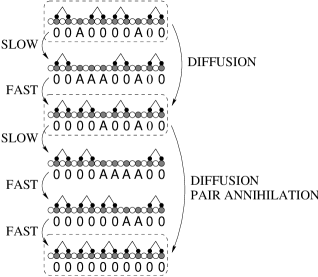
Figure 9: Time evolution of a state, consisting of attachment (fast) and detachment (slow) events. The coarse-grained interpretation includes only long-living states (in boxes). The effective steps include diffusion, pair annihilation and pair creation (not shown).
© 2001, EDP Sciences vilfan2001b

Table 3: The processes in the $A+A\leftrightarrow 0$ model onto which the stiff dimer model can be mapped in the limit $K\gg 1$.

	Process	Rate	Branching	Total
		(1)	prob. (2)	rate
Hopping	$A00\stackrel{{\scriptstyle(1)}}{{\to}}AAA\stackrel{{\scriptstyle(2)}}{{\to}}A00$	$k_{-}$	$\frac{1}{2}$	$\frac{k_{-}}{2}$
Annihilation	$A00A\stackrel{{\scriptstyle(1)}}{{\to}}AAAA\stackrel{{\scriptstyle(2)}}{{\to}}\left\{\begin{array}[]{c}00AA\\ AA00\end{array}\right\}\to 0000$	$k_{-}$	$\frac{2}{3}$	$\frac{2k_{-}}{3}$
Creation	$0000\stackrel{{\scriptstyle(1)}}{{\to}}\left\{\begin{array}[]{c}00AA\\ AA00\end{array}\right\}\stackrel{{\scriptstyle(2)}}{{\to}}AAAA\stackrel{{\scriptstyle(2)}}{{\to}}A00A$	$k_{-}$	$\frac{k_{-}}{k_{-}+k_{+}}\times\frac{1}{3}$	$\frac{k_{-}}{3K}$

Then processes like $A00\to AAA\to 00A$ result in an effective diffusion for particle $A$ with a hopping rate $r_{\rm hop}=k_{-}/2$ ($k_{-}$ is the rate of the first transition and $1/2$ the branching probability for the second) and an effective step width of two lattice sites. The hopping rate is different for the last step before two particles annihilate ($A00A\to 00AA$), namely $k_{-}/3$. Pair annihilation, $AA\rightarrow 00$, occurs with a rate $k_{+}c$, or $2k_{-}/3$ from the state $A00A$. Pair creation, on the other hand, occurs mainly through the process $0000\to 00AA\to AAAA\to A00A$; the corresponding rate is $k_{-}/3K$ per lattice site and hence largely suppressed with respect to the annihilation process as long as the particle concentration is far above its steady-state value. These processes are summarized in Tab. 3. Other processes involve more particles and are of higher order in terms of a power series in $K^{-1}$. They are negligible if the number of vacancies is small, $n_{A}\ll 1$, and the binding constant is large, $K\gg 1$. In summary, for $K\gg 1$, our dimer model can be mapped onto a one-particle reaction-diffusion model $A+A\rightarrow 0$. Pair creation processes, $0\rightarrow A+A$, are highly suppressed during the first stage of the relaxation process. The give a significant contribution to the dynamics close to the steady state where the relaxation becomes exponential instead of algebraic.

Models like the simple reaction-diffusion model $A+A\rightarrow 0$ show interesting non-equilibrium dynamics privman97 ; mattis98 ; schuetz98 . One can show torney83 ; toussaint83 that asymptotically the particle density $n_{A}(t)$ decays algebraically, $n_{A}(t)\propto t^{-1/2}$, which nicely explains the slow decay observed in simulation data (see Fig. 8). Note that a mean-field like rate equation

$$\partial_{t}n_{A}(t)\propto-n_{A}^{2}(t)$$ (29)

would predict $n_{A}(t)\propto t^{-1}$. In our analysis we can even go beyond the asymptotic scaling analysis and try to compare with exact solutions of the model for a random initial distribution with density $p$ by Krebs et al. krebs95 . They find (adapted to our situation with two-site hopping)

$$n_{A}(t)=\frac{1}{2\pi}\int\limits_{0}^{2}du\,\frac{\sqrt{u(2-u)}\,\left(n_{0}^{\rm plateau}\right)^{2}\,e^{-16ur_{\rm hop}t}}{u\,\left(u(\frac{1}{2}-{n_{0}^{\rm plateau}})+\left(n_{0}^{\rm plateau}\right)^{2}\right)}\;.$$ (30)

Its asymptotic limit (first determined by Torney and McConnel torney83 ) reads

$$n_{A}=(32\pi r_{\rm hop}t)^{-1/2}$$ (31)

Note that it is independent of the initial particle concentration in the Flory plateau ${n_{0}^{\rm plateau}}$.

Our Monte-Carlo data (see Fig. 8) are in excellent agreement with the predictions of Eq. 30. Minor deviations at times between the plateau and the power-law decay are due to the assumption of a random particle distribution underlying the derivation of Eq. 30. In reality the state after initial binding (RSA) contains some correlations which however do not reach beyond a vacancy (Markov-shielding) evans93 . In other words, the sizes of occupied areas are not exponentially distributed, but they are uncorrelated to each other and the higher-order correlation functions decay as fast as 2-point correlations (super-exponentially). Short ranged correlations in the initial configuration do have some effect on concentration at intermediate times and this causes the deviation between the simulation data and the theoretical curve which, however, is not large. According to family91 ; santos97 correlations can affect the concentration in the asymptotic limit even if the pair correlation function is short ranged and the order-$n$ correlation functions decay at a length-scale of $\mathcal{O}(n)$, but this is not the case in our model.

The results from the $A+A\rightarrow 0$ model also become invalid for very long times where the particle concentration comes close to its equilibrium value. In this limit the dynamics becomes scale-invariant racz85 . The particle concentration can be written in scaling form

$$n_{A}(t)=K^{-1/2}\hat{n}(k_{-}t/K)$$ (32)

with a diverging characteristic time scale $\tau_{K}\propto K$.

IV.1.4 Steady-state autocorrelation functions

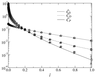
Figure 10: Scaled equilibrium autocorrelation functions for $\hat{C}_{0}(\hat{t})=KC_{0}(t)$, $\hat{C}_{D}(\hat{t})=C_{D}(t)$ and $\hat{C}_{P}(\hat{t})=KC_{P}(t)$ , $\hat{t}=k_{-}t/K$. The function $\hat{C}_{P}(\hat{t})$ is compared with the analytical result (39), represented by the solid line. Simulation data were obtained with $K=100$ (circles, for $C_{0}$ and $C_{D}$ connected with dot-dashed and dashed lines) and $K=400$ (triangles).
© 2001, EDP Sciences vilfan2001b

A limitation of the above mapping becomes evident if one considers the equilibrium autocorrelation functions. Contrary to conventional $A+A\leftrightarrow 0$ models there are three different autocorrelation functions with different functional forms (Fig. 10). In the following we will use $\hat{n}_{(i,i+1)}$ as the occupation number (0 or 1) of a dimer on the pair of sites $(i,i+1)$ and $\hat{n}_{0_{i}}$ as the occupation number of a vacancy at the site $i$ (1 if there is a vacancy, 0 otherwise). The dimer autocorrelation function

$$C_{D}(\tau)=\left<\hat{n}_{(i,i+1)}(t)\hat{n}_{(i,i+1)}(t+\tau)\right>-\left<\hat{n}_{(i,i+1)}(t)\right>^{2}$$ (33)

describes the probability to find a dimer at a given pair of sites simultaneously at times $t$ and $t+\tau$. Similarly we define the vacancy autocorrelation function

$$C_{0}(\tau)=\left<\hat{n}_{0_{i}}(t)\hat{n}_{0_{i}}(t+\tau)\right>-\left<\hat{n}_{0_{i}}(t)\right>^{2}$$ (34)

describing the probability that the site $i$ is vacant at times $t$ and $t+\tau$. To calculate their values at $\tau=0$, we need the expectation values

$$\left<\hat{n}_{(i,i+1)}(t)\right>=\left<\hat{n}^{2}_{(i,i+1)}(t)\right>=n_{D}=\frac{1}{2}\left(1-\frac{1}{\sqrt{4K+1}}\right)$$ (35)

and

$$\left<\hat{n}_{0_{i}}(t)\right>=\left<\hat{n}^{2}_{0_{i}}(t)\right>=n_{0}=\frac{1}{\sqrt{4K+1}}\;.$$ (36)

A third way of defining an autocorrelation function is to ask for the probability that a vacancy is either on the site $i$ or on the site $i+1$

$$C_{P}(\tau)=\Bigl{<}(\hat{n}_{0_{i}}+\hat{n}_{0_{i+1}}-\hat{n}_{0_{i}}\hat{n}_{0_{i+1}})(t)\times\\ \times(\hat{n}_{0_{i}}+\hat{n}_{0_{i+1}}-\hat{n}_{0_{i}}\hat{n}_{0_{i+1}})(t+\tau)\Bigr{>}\\ -\left<(\hat{n}_{0_{i}}+\hat{n}_{0_{i+1}}-\hat{n}_{0_{i}}\hat{n}_{0_{i+1}})(t)\right>^{2}\;,$$ (37)

with

$$\left<\hat{n}_{0_{i}}+\hat{n}_{0_{i+1}}-\hat{n}_{0_{i}}\hat{n}_{0_{i+1}}\right>=\frac{2n_{0}}{1+n_{0}}=\frac{2}{\sqrt{4K+1}+1}\;.$$ (38)

The important difference between $C_{P}$ and $C_{0}$ originates from the fact that the vacancies diffuse by hopping over two lattice sites. This is why a vacancy diffusing along odd sites will not influence the function $C_{0}$ if the original vacancy was on an even site. The function $C_{P}$ does not make this distinction.

For $K\gg 1$ the autocorrelation functions become scale invariant as well. Their scaling form reads $\hat{C}_{0}(\hat{t})=KC_{0}(t)$, $\hat{C}_{D}(\hat{t})=C_{D}(t)$ and $\hat{C}_{P}(\hat{t})=KC_{P}(t)$ with $\hat{t}=k_{-}t/K$. The latter corresponds to the autocorrelation function in a reaction-diffusion model $A+A\leftrightarrow 0$, which has recently been calculated analytically by Bares and Mobilia bares99

$$\hat{C}_{P}(\hat{t})=\left(\frac{e^{-2\hat{t}}}{\sqrt{2\pi\hat{t}}}-\mbox{Erfc}\,\sqrt{2\hat{t}}\right)\mbox{Erfc}\,\sqrt{2\hat{t}}\;,\\ {\rm with}\quad\mbox{Erfc}\,(x)=\frac{2}{\sqrt{\pi}}\int_{x}^{\infty}e^{-y^{2}}dy\;.$$ (39)

Note that the described solution is derived for a parameter set which requires a special relation between diffusion, pair-creation and annihilation rate to be fulfilled. In our model this is not the case. But, this difference becomes irrelevant in the scaling limit, since their and our model can be mapped onto each other by introducing a short-ranged interaction between particles. See also Ref. park01 for a comment about the validity of the analytical approximation used in Ref. bares99 . The observed deviations however do not affect the scaling limit.

The other two functions decay on the same time-scale, but with different prefactors. The reason is that even if a pair of vacancies annihilates, the system still keeps memory on whether the surrounding dimers were located on even or odd locations and this gives those correlation functions that distinguish between even and odd sites a longer decay time.

IV.2 Two-particle model

Another interesting case arises if we consider the limit $K_{2}\to\infty$ with $K_{1}c$ being of the order of magnitude $1$. In this case neither the dimers bound with one head nor the empty lattice sites dominate and we have to introduce two particle types. As we are used to, particles $A$ should denote vacancies on the lattice. In addition, we introduce particles $B$, representing dimers bound with only one head.

Reactions $A\to B$ and $B\to A$ occur at rates $k_{1+}c$ and $k_{1-}$. If we assume that both attachment rates of the second head $k_{2+}^{f}$ and $k_{2+}^{b}$ are significantly higher than $k_{1+}c$ and $k_{1-}$, we are again dealing with the diffusive model (25). The diffusion mechanism for vacancies (particles A) is exactly the same as in the model with stiff dimers and according to (24) the hopping rate is given by Eq. (24). The diffusion rate of single-bonded dimers (particles B) has to be equal. This is due to the symmetry of our model upon exchanging particles A and B and the transition rates $k_{1+}c$ and $k_{1-}$ (Tab. 1) and because the latter are irrelevant for the hopping rate. If a particle A and a particle B reach neighboring sites, they annihilate quickly, while two particles of the same type do not interact. To summarize, we obtain a reaction diffusion model of the type:

$$A \leftrightarrow B$$

$$A+B \leftrightarrow 0$$

While its dynamics is more complex at short times, the model becomes equivalent to the $A+A\leftrightarrow 0$ if the transitions between $A$ and $B$ become faster than the typical annihilation time, which is given as the diffusion time between two particles, displaced by the average distance between particles on the lattice, $\sim\frac{1}{r_{\rm hop}n^{2}}$. Therefore the power-law behavior, given by (31) remains untouched by the fact that we are dealing with two different particle types. An example of a simulation in this regime is shown in Fig. 11.

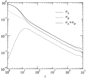
Figure 11: A computer simulation showing the time dependence of the vacancy ($n_{A}$) density, the single-bonded dimer ($n_{B}$) density and their sum for $K_{1}c=0.5$ and $K_{2}=10^{6}$. The dotted line shows the predicted long-time limit of reaction-diffusion models given by Eq. (31). In detail, parameters are: $k_{+1}c=0.1$, $k_{-1}=0.2$, $k_{+2}^{f}=10^{6}$, $k_{-2}^{f}=1$, $k_{+2}^{b}=0.1\,k_{+2}^{f}$ and $k_{-2}^{b}=0.1\,k_{-2}^{f}$. The simulation has been performed on a lattice with $2^{14}$ sites and periodic boundary conditions.

IV.3 Dynamics of interacting dimers in one dimension

In many biological systems the interaction between attached molecules plays an important role. For example, in the case of kinesin, there has been an observation of coexisting empty and decorated domains which can only be explained by an attractive interaction vilfan2001a . Similar observation has been made on actin decorated with double-headed myosin orlova97 . An interaction between the dimers can be introduced by assuming that a dimer is more likely to bind to a pair sites if one or two neighbors are already bound. The binding rate then becomes $k_{+}^{P}=k_{+}^{N}=Ak_{+}^{N}$ (one neighbor bound) or $k_{+}^{D}=A^{2}k_{+}^{N}$ (both neighbors bound). Similar, we assume that a dimer with one bound neighbor dissociates with rate $k_{-}^{P}=k_{-}^{M}=Bk_{-}^{N}$ and that a dimer with two bound neighbors dissociates with rate $k_{-}^{D}=B^{2}k_{-}^{N}$. The equilibrium state of this model is still exactly solvable mcghee74 , but the interaction changes both relaxation stages quantitatively. First, the vacancy concentration on the intermediate plateau lowers since the interaction improves the formation of contiguous clusters during the first stage. The RSA phase can then be described in terms of Kolmogorov’s grain-growth model kolmogorov37 . The vacancy concentration after the initial binding is given as $n_{0}\approx\frac{1}{2}\sqrt{\frac{\pi r_{\rm nuc}}{2r_{\rm growth}}}$ gonzalez74 ; evans83 , where $r_{\rm nuc}$ is the nucleation rate per free lattice site (in the simplest case, when $K\gg 1$, it is simply $k_{+}$) and $r_{\rm growth}$ the sum of speed with which both boundaries of a nucleus spread over the lattice (normally $k_{+}^{P}+k_{+}^{M}=2Ak_{+}^{N}$). The second effect of the interaction is that the diffusional relaxation slows down by the factor $B$ since the detachment rate decreases. And finally, the equilibrium vacancy concentration decreases mcghee74 . Nevertheless, interacting models show the same two-stage relaxation behavior. An example of a model with interaction is shown by the dot-dashed line in Fig. 12.

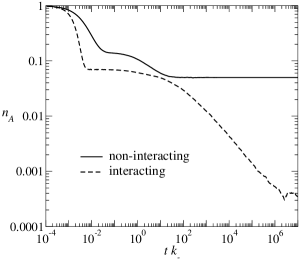
Figure 12: The number of vacant lattice sites as a function of time non-interacting (solid line) and interacting (dashed lines) dimers. The parameters were $K=100$, $A=10$ and $B=1/10$ (a dimer is 10 times as likely to associate to and 10 times less likely to dissociate from a certain site if one of the neighbors is present)

V Dimer model with interaction

As we mentioned in Section IV.3, interactions between bound dimers can often play an important role. In the kinesin-microtubule system, evidence for the existence of an attractive interaction comes from two key experimental observations. The first one is that bound kinesin dimers are found to form two-dimensional crystalline lattices thormaehlen98 . Within the non-interacting model one can explain longitudinal correlations along a single protofilament, but by no means the alignment of dimers on different protofilaments. The second observation supporting an attractive interaction between bound dimers is the coexistence of empty and decorated microtubules in one and the same experiment vilfan2001a . Such a phase segregation is a clear indication that the system is in a coexistence regime with the strength of the dimer interaction above some critical value. The detailed nature of the interaction between the dimers is not yet known. It could be a direct interaction between kinesin heads and tails or some indirect interaction mediated through distortions of the underlying tubulin lattice or a combination of all of these possibilities. All of these mechanisms are consistent with the observation that the interaction is stronger on flat tubulin sheets than on cylindrical microtubules vilfan2001a .

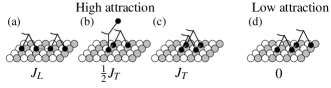
Figure 13: Illustration of the interaction energy between two adsorbed dimers in different relative positions.
© 2001, Academic Press vilfan2001a

Even if one assumes that there is only nearest-neighbor interaction, a general description would still require $12$ different coupling strengths ($2$, $4$ and $6$ for describing the attraction between two single-bonded dimers, two double-bonded dimers and between a single- and a double-bonded dimer, respectively). Upon neglecting that the tubulin lattice is actually rhombic and not orthogonal one can reduce the number of different coupling constants to $9$. These are still too many for a general discussion. Hence, mainly for simplicity, we will restrict ourselves to a model with only two interaction constants, $J_{L}$ acting in longitudinal and $J_{T}$ acting in transverse direction, as illustrated in Fig. 13. We assume that the interaction between two double-bonded dimers on neighboring protofilaments is zero if they are displaced by one lattice site or more (Fig. 13d). Otherwise, the transverse interaction is assumed to have the strength $J_{T}$ between two double-bonded dimers (Fig. 13c) and $\frac{1}{2}J_{T}$ between a double- and a single-bonded dimer (Fig. 13b). We use the same notation as in Sec. IV.3 and introduce factors $A_{i}$ and $B_{i}$ measuring the change in the attachment and detachment rate by the presence of a neighboring dimer (with $i$ indicating the relative position of the neighbors as shown in Fig. 13),

$$k_{1,2+}^{\text{with neighbour}} =A_{i}\,k_{1,2+}^{\text{without neighbour}}\;,$$

$$k_{1,2-}^{\text{with neighbour}} =B_{i}\,k_{1,2-}^{\text{without neighbour}}\;.$$

Detailed balance states that

$$J_{i}=k_{B}T\ln\frac{A_{i}}{B_{i}}\;.$$ (40)

For simplicity we further assume that the binding and the unbinding rate are always changed by the same factor, $A_{i}=1/B_{i}$; this assumption is irrelevant in equilibrium, but it simplifies the kinetics.

Fig. 14 shows the stoichiometry curves, equivalent to those in Fig. 6, for the interacting model. The most dramatic effect of the interaction is that it broadens the plateau where most dimers are double-bonded, giving a stoichiometry of one head per lattice site. If the interaction is strong enough (see e.g. the curve with $J/k_{B}T=2$ in Fig. 14), the stoichiometry curves show quite a steep rise from zero to the plateau at $\nu=1$. This is quite indicative of a phase transition, albeit smeared somewhat out due to finite-size effects.

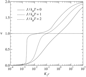
Figure 14: Binding stoichiometry of the interacting dimer model (dashed lines) compared with the non-interacting (solid line). The binding constant of the second head is $K_{2}=10$, the interaction strength $J=J_{T}=J_{L}=k_{B}T$ (short-dashed line) and $2\,k_{B}T$ (long-dashed line).

To determine the critical point we make two further simplifications. First, we assume that we are in the stiff dimer limit, $K_{2}\gg 1$, as we did in Sec. IV.1. This stiff dimer model can be interpreted as a spin model with axial next nearest neighbor interaction, also known as ANNNI models, reviewed by Selke selke88 . In terms of these ANNNI models, our model is a rather peculiar limit since it has an infinitely repulsive interaction between nearest neighbors and attractive interaction between next-nearest neighbors in longitudinal direction, as well as an attractive interaction between nearest neighbors in transverse direction. In the literature on ANNNI models mainly the opposite situation was studied since it leads to frustrations, while the “zero-temperature” state of our model is trivial, namely dimers aligned, let us say, the even sites on the protofilaments. This justifies an approximation which further simplifies the model, namely by assuming that dimers can only bind to even sites. Then the problem simplifies to a lattice-gas model with an effective Hamiltonian

$$\mathcal{H}=\sum_{i,j}\left(-J_{L}\hat{n}_{2i,j}\hat{n}_{2i+2,j}-J_{T}\hat{n}_{2i,j}\hat{n}_{2i,j+1}-\mu\hat{n}_{2i,j}\right)\;,$$ (41)

where the coordinates $(2i,j)$ run over all even lattice sites, $\hat{n}_{2i,j}$ are the occupancy numbers ($0$ or $1$) on those sites and $\mu=k_{B}T\ln(K_{1}K_{2}c)$ is the chemical potential of adsorbed dimers. The lattice gas model can be mapped onto the 2D Ising model yeomans92 with Hamiltonian

$$\mathcal{H^{\prime}}=\sum_{i,j}\left(-J^{\prime}_{L}s_{i,j}s_{i+1,j}-J^{\prime}_{T}s_{i,j}s_{i,j+1}-\epsilon s_{i,j}\right)$$ (42)

with exchange constants

$$J_{T}^{\prime}=\frac{1}{4}J_{T}\,,\qquad J_{L}^{\prime}=\frac{1}{4}J_{L}\,,$$ (43)

and spin variables

$$s_{i,j}=2\hat{n}_{2i,j}-1\;.$$ (44)

The spin $s$ has the value $+1$ if it is parallel and $-1$ if it is antiparallel to the magnetic field $\epsilon$,

$$\epsilon=\frac{\mu+J_{L}+J_{T}}{2}\;.$$ (45)

The critical temperature of the two dimensional Ising model was first determined by Kramers and Wannier kramers41 . In the absence of an external field, the model has also been exactly solved by Onsager onsager44 . The condition for the critical point reads

$$\sinh\frac{J_{L}}{2k_{B}T}\times\sinh\frac{J_{T}}{2k_{B}T}=1\;,$$ (46)

or $J_{c}=1.76\,k_{B}T$ in the isotropic case ($J_{L}=J_{T}$).

The exact solution helps us to determine the critical point, i.e. the interaction strength needed to obtain a phase transition between an empty and a decorated state. The full form of the binding stoichiometry as a function of concentration, however, would be equivalent to calculating the magnetization of the two-dimensional Ising model in the presence of an external field, which has not yet been achieved analytically. Therefore, one has to rely on computer simulations to obtain the stoichiometry curves. An overview on Monte-Carlo simulations on lattice gas models can be found in Ref. binder89 . The situation simplifies when one is far away from the critical point, i.e. when the coupling is much stronger than its critical value, $J\gg J_{c}$. This corresponds to the low-temperature limit in the Ising analogue, where the spin polarization is saturated and points into the direction of the external field. The number of spins with orientation $\uparrow$ is given as $n=N\Theta(\epsilon)$, where $\Theta$ is the Heaviside function. Back in the adsorption model, according to Eqs. (43)-(45), the condition reads

$$\nu=\Theta(\mu+J_{L}+J_{T})\;.$$ (47)

This expression can also be understood directly. The boundary of a decorated domain will normally consist of many edge elements (each one with three out of four neighboring sites occupied) and some corner elements (with two out of four neighboring sites occupied). If the corner elements are stable, the decorated domain will grow; if they are unstable, it will shrink. The stability condition of a corner element with one bound longitudinal neighbor and one bound transverse neighbor is given by Eq. (47). Deviations from (47) are possible due to finite size effects. This is because small patches have a higher curvature in the boundary and are therefore less stable.

V.1 Dynamics of the interacting 2D model

We have shown in Sec. IV.1.3 that the annealing of gaps between bound dimers can be slowed down substantially as compared to the transition rates for single dimers. This effect is even stronger in a two dimensional system. Here linear domain boundaries emerge instead of point defects (gaps). These boundaries can annihilate when two of them join. But their diffusion is significantly slower than the diffusion of single gaps, roughly inverse proportional to the number of sites in the boundary.

The nonequilibrium dynamics of decorating an initially empty two-dimensional lattice is an interesting and complex problem. It has first been studied by Becker and Döring becker35 (reviewed in Ref. lewis78 ). A crucial concept is the critical nucleus, a certain number of adsorbed atoms (here dimers) necessary to form a stable nucleus able to grow and spread over the whole lattice. An analytical expression for the nucleation time can be given if the interaction is strong enough, and the critical cluster size becomes as small as four, three or two molecules. For larger critical cluster sizes a rough estimate says that the nucleation rate is proportional to the kinesin concentration to a power that is typically half the number of nucleus-forming units.

There are different scenarios depending on the relative magnitude of the time to form a critical nucleus, $t_{\rm nuc}$, and its growth time, $t_{\rm growth}$, i.e. the time it takes such a nucleus to grow and cover the whole surface (see Fig. 15a). If the nucleation time is larger than the growth time,

$$t_{\rm nuc}\gtrsim t_{\rm growth}\;,$$ (48)

the whole lattice will most probably be completely covered with dimers before other nucleation sites can form anywhere else on the lattice. The final state is a defect free lattice generated from a single nucleus. This is consistent with experimental observations thormaehlen98 . At the same time single-site nucleation also explains how empty and fully decorated microtubules can be found coexisting in one and the same experiment vilfan2001a . When the decoration starts, nuclei will form on certain microtubules and totally decorate them, until the concentration of free kinesin in solution drops below the critical value, where the equilibrium phase is the empty lattice. A numerical study of the nucleation process vilfan2001a gives us an estimate of the minimum interaction strength needed to fulfill the condition (48) as $J\approx 3\,k_{B}T$. This strongly indicates that there is a interaction between kinesin dimers which is of the order of $3\,k_{B}T$.

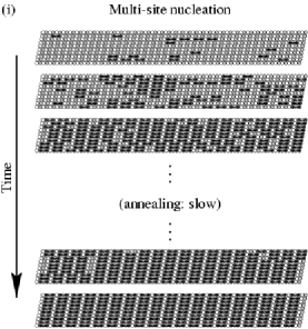
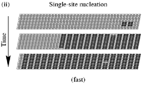
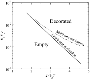
a)	b)

Figure 15: a) Computer simulation of (i) multiple-site nucleation with subsequent annealing and (ii) single-site nucleation. Both processes can lead to a defect-free decoration. However, annealing can be extremely slow whereas single-site nucleation immediately leads to the ordered state. The parameters in the simulation were the following: (i): $K_{1}K_{2}c=0.1$, $A_{L}=A_{T}=3$, $B_{L}=B_{T}=0.3$ (ii): $K_{1}K_{2}c=0.001$, $A_{L}=A_{T}=10$, $B_{L}=B_{T}=0.1$. b) The solid line shows the phase transition above which a decorated phase exists. The dashed line shows the border between homogeneous (defect-free) decoration reached immediately through nucleation and decoration with domain walls. The curves were obtained from a computer simulation on a lattice of $14\times 100$ sites (note that the defect-free range would be somewhat larger on a smaller lattice).
© 2001, Academic Press vilfan2001a

If the nucleation time is smaller than the growth time,

$$t_{\rm growth}\gtrsim t_{\rm nuc}\;,$$ (49)

there is a certain probability that a second critical nucleus forms on the lattice before the first one created had a chance to cover the whole lattice. The probability of such or higher order events grows with decreasing nucleation time. Then, the lattice will be covered by several domains, locally ordered areas which may be out of phase on the microtubule lattice. In order to finally reach a homogeneous decoration with only one predominant domain a secondary process is needed which leads to a coarsening of the initial grain-like structure. This secondary process includes domain wall wandering and annihilation induced by the detachment and re-attachment of kinesin dimers. As mentioned above, such annealing processes are expected to be much slower than the unhindered growth of individual domains. Fig. 15b summarizes the possible phases and dynamic regimes for interacting dimers decorating a two-dimensional lattice.

VI Interacting $k$-mers in one dimension

Non-interacting $k$-mers ($k>3$) are well described with the mean-field kinetics of the model $kA\to 0$ which predicts a gap density decay $\propto t^{-1/(k-1)}$ nielaba92 ; privman92a . In the continuous limit, also called continuous sequential adsorption (CSA) or “car parking problem” the length of unoccupied space decays as $\propto 1/\log t$ in the mean-field regime krapivsky94 ; jin94 .

The dynamics becomes more intriguing when a strong attraction between the $k$-mers is introduced. An example of such a system is tropomyosin vilfan2001c , a protein that plays a key role in the regulation of muscle contraction. In muscle each tropomyosin molecule binding on an actin filament occupies seven actin monomers (although other isoforms covering 5 or 6 monomers exist as well hitchcock-degregori94 ) and thereby obstructs the action of myosin motors. The binding of tropomyosin to actin is strongly cooperative – the binding constant next to a bound molecule is 1000 times larger than at an isolated place wegner79 .

The initial binding phase is analog to the problem of interacting dimers and can again be described using a grain growth model kolmogorov37 ; evans93 ; vilfan2001c . After the initial phase, gaps with sizes between $1$ and $k-1$ sites will remain. Their sizes are distributed randomly with equal probabilities of $1/(k-1)$ for each gap size. What follows is again a process on a much longer time-scale in which $k$-mers at edges of the gaps can detach and re-attach. If they detach from one side of the gap and then re-attach at the other side, the gap moves by $k$ sites in one direction (see Fig. 16a).

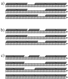
Figure 16: Examples of effective reactions that occur after the detachment and attachment of a heptamer: Diffusive step (a); Pair coagulation $A+A\to A$ (b); Pair annihilation $A+A\to 0$ (c).
© 2001, Biophysical Society vilfan2001c

The rate of such diffusive steps is given as the detachment rate of a molecule on e.g. the minus side of a block multiplied by the probability that a molecule re-attaches on the plus side of the neighboring block before another $k$-mer can re-attach to the position where the first one has detached:

$$r_{\rm hop}=k_{-}^{M}\frac{k_{+}^{P}}{k_{+}^{P}+k_{+}^{M}}=k_{-}^{M}\frac{k_{-}^{P}}{k_{-}^{P}+k_{-}^{M}}=\left(\frac{1}{k_{-}^{P}}+\frac{1}{k_{-}^{M}}\right)^{-1}\;.$$ (50)

Two neighboring gaps (see Figs. 16b and c), each containing between $1$ and $k-1$ sites with randomly distributed probabilities, can either join to a single gap (Fig. 16b) or, if their total size exactly fits one $k$-mer, annihilate (Fig. 16c). If the original gap sizes are $g_{1}$ and $g_{2}$, the joined gap has size $(g_{1}+g_{2})\mod k$. The annihilation will take place in $k-1$ out of $(k-1)^{2}$ cases, therefore its probability is $1/(k-1)$. Any other gap size will be the outcome in $k-2$ cases, therefore having the probability $(k-2)/(k-1)^{2}$.

Again we can represent gaps as particles $A$ hopping randomly along the lattice and joining or annihilating when two of them meet. The pair creation processes become relevant only if the particle concentration approaches its equilibrium value and will be neglected for now. Then, we can map our model to a diffusion-coagulation-annihilation model consisting of following reactions

$$A+A \to A \;(k-2)/(k-1)\;,$$ with probability

$$A+A \to 0 \;1/(k-1)\;.$$ with probability

The fundamental difference between the interacting $k$-mer and the dimer model is that the $k$-mer model not only contains pair annihilation but also pair coagulation processes, $A+A\to A$. According to Ref. lee94 all diffusion-annihilation models of the type $2A\to lA$ (or generally $mA\to lA$) belong to the same universality class. In the asymptotic limit, the “particle” concentration can then be borrowed from the exactly solvable $A+A\to 0$ model lushnikov87 ; torney83 . Adapted to our $k$-mer model it reads

$$n_{A}(t)=\frac{2}{2-l}\frac{1}{\sqrt{8\pi\bar{r}_{\text{hop}}t}}$$ (51)

with $l=(k-2)/(k-1)$ and $\bar{r}_{\text{hop}}=k^{2}r_{\text{hop}}$; the second relation results from the fact that in each diffusive step a gap jumps over $k$ sites. Hence, we finally obtain

$$n_{A}(t)=\frac{k-1}{k^{2}\sqrt{2\pi r_{\text{hop}}t}}\;.$$ (52)

Interestingly, the asymptotic particle concentration is independent of its initial value, i.e. the final gap concentration at long times does not depend on the intermediate gap concentration $n_{A}^{0}$. Note that it is even independent of the solution concentration $c$.

Figure 17: The time-dependent gap concentration ($n_{G}$) and fraction of empty lattice sites ($n_{0}$) for an interacting pentamer ($k=5$), as obtained from the simulation. The dot-dashed line shows the prediction of Eq. (52) and the dotted line the mean-field power law $\propto t^{-1/(k-1)}$. The thin solid and dashed line show the equilibrium values of $n_{G}$ and $n_{0}$ using the expression from Ref. mcghee74 . The parameters are: $k_{+}^{N}c=100$, $k_{+}^{P}c=k_{+}^{M}c=1000$, $k_{-}^{N}=1$, $k_{-}^{P}=k_{-}^{M}=0.1$, $k_{+}^{D}c=10000$ and $k_{-}^{D}=0.01$.

Of course, the mapping to the $A+A\to lA$ model is valid only as long as the concentration of particles $A$ is well above its equilibrium concentration. Otherwise, particle splitting events like $A\to A+A$ also become relevant. If the concentration $c$ is high enough, the $t^{-1/2}$ regime will be followed by a regime where, due to these splitting events, the average gap size will finally approach one site, which then are randomly distributed over the lattice. The number of gaps will decay according to the mean-field prediction $\propto t^{-1/(k-1)}$, as it does in the non-interacting $k$-mer model nielaba92 ; privman92a . An example of this behavior is shown in Fig. 17. When the system approaches equilibrium, processes of pair creation $0\to A+A$ become important as well. Similar to the dimer model, these processes leads to a final exponential relaxation towards equilibrium. The equilibrium gap size and distribution of the interacting $k$-mer model are known exactly from a study by McGhee and von Hippel mcghee74 .

VII Summary and Outlook

In this contribution we have discussed the kinetics of some macromolecular assembly processes relevant for the formation of functional structures in cells. In particular, we were interested in the dynamics of ligand-substrate binding, where the substrate is a one- or two-dimensional lattice and the ligands are dimers or oligomers. As examples we picked binding of dimeric kinesin on microtubules and tropomyosin on actin filaments. There are other related systems where protein ligands bind to biological macromolecules, e.g. proteins to DNA or antibodies to viruses.

Our theory allows us to study the effects of steric constraints, binding rates and interaction between neighboring proteins on the binding dynamics and binding stoichiometry. Our key results are as follows. The collective dynamics turns out to be not only much slower than the kinetics of single molecules but it also shows some interesting dynamic anomalies. Quite generally, we find that the binding kinetics goes through several qualitatively different stages. At small times when deposition processes are frequent but detachment processes are still unlikely, the kinetics can be described in terms of sequential deposition models. Such models have been analyzed in various contexts years ago so that there are many exact results available. After this initial phase the system is left in a “metastable” or “locked” configuration, i.e. a configuration with many small vacant regions between blocks of bound molecules prohibiting binding of additional ligands to the substrate. As a consequence one obtains an intermediate plateau regime for the binding stoichiometry. For escaping from this locked configuration vacant regions have to merge in order to accommodate for the deposition of additional ligands. These are extremely slow processes mediated by a sequence of detachment and re-attachment processes. Upon identifying the gaps with particles $A$ we have shown that the dynamics in this regime can be explained by mapping it onto reaction-diffusion models. For stiff dimers the corresponding model is $A+A\rightarrow 0$ resulting in a gap density that decays with a power law $\propto t^{-1/2}$ before it approaches the final equilibrium value. Taking into account that actual biological dimers have some level of flexibility the model had to be generalized to include a second species of particles $B$, representing dimers bound with only one head. The corresponding reaction-diffusion model is then of the type $A\leftrightarrow B$ and $A+B\leftrightarrow 0$. While its dynamics is more complex at short times, the model becomes equivalent to the $A+A\leftrightarrow 0$ if the transitions between $A$ and $B$ become faster than the typical annihilation time. If, on the other hand, one introduces a strong diffusion of adsorbed dimers the power-law decay is preceded by a mean-field regime where the gap density decays with $\propto t^{-1}$. The two-stage relaxation and the mapping to the $A+A\to 0$ model remain valid even if there is an attractive interaction between adsorbed dimers on the one-dimensional lattice. In the two-dimensional model with interaction, the sequential deposition stage goes over into a nucleation process and the relaxation stage into a much slower annealing process. Yet even then the two-stage relaxation remains qualitatively the same.

The annealing process for interacting $k$-mers with $k>3$ is fundamentally different from the dimer model. One finds that non-interacting $k$-mers are always well described with the mean-field kinetics of the model $kA\rightarrow 0$ predicting a decay in the gap density $\propto t^{-1/(k-1)}$. Introducing a strong interaction between the $k$-mers, as is the case for tropomyosin binding on actin filaments, we find a mapping to the $A+A\rightarrow lA$ model, valid for concentrations well above the equilibrium value, which shows a particle concentration decaying $\propto t^{-1/2}$. Closer to equilibrium other processes become important as well. First, particle splitting, $A\to A+A$ leads to an intermediate mean-field regime similar to that of non-interacting $k$-mers. Later the events of pair creation, $0\to A+A$ become relevant and lead the system into the final exponential relaxation towards equilibrium.

All of the above results concern the statics and dynamics of ligands decorating periodic structures in the absence of ATP hydrolysis. Such systems are “passive” in the sense that the ligands bind and unbind from their respective substrates but do not show any motor activity, i.e. move along these molecular tracks. As described above, this allowed us to give a detailed description of decoration experiments and to analyze corresponding experiments quantitatively. We also were able to identify and quantify cooperative effects between kinesin dimers. As our results show, the relaxation time in many experimental or biological systems can be extremely long. Therefore, one has to be aware that an experiment where the measurement is taken soon after the start of the decoration often does not show the equilibrium configuration, but rather some intermediate state from the relaxation process.

A natural extensions of this work is to investigate “active” systems composed of an ensemble of motor proteins and their respective substrates in the presence of transport along the molecular tracks driven by the chemical energy of ATP hydrolysis. Understanding such systems lies at the heart of many cellular processes. Although single processive motors like kinesin or myosin V can move loads over considerable distances, the number of motors acting simultaneously when transporting vesicles through the cytoplasm can be pretty large. For instance, in Ref. feneberg2001 the force acting on a bead in the cell has been estimated as $100-200\,{\rm pN}$, which implies that at least $20-40$ motor proteins were involved. How these active motors cooperate at high densities and what role is played by interactions between them, is to a large extend a still unexplored field with many open questions.

An even broader range of questions arises when one tries to understand how cells organize their interior to fulfill their various duties. While organizing its interior, the cell has to physically separate molecules or molecular aggregates from each other, define distinct functional regions, and actively transport molecules between these regions. Such processes rely on the assembly and ordering processes of macromolecules inside the cell and on forces that may be generated by molecular assembly or by the action of motor proteins. Understanding the principles underlying those complex cellular processes not only requires biological and biochemical studies but also studies of physical processes. In this respect microtubules and motors have been used as in vitro model systems to study various aspects of regulation and self-organization of cellular structures. It was shown theoretically and experimentally that the dynamic instability of microtubules in combination with microtubule polymerization forces is sufficient to provide a microtubule organizing center with a mechanism to position itself at the center of a confined geometry holy97 ; dogterom97 . In a simple in vitro system consisting solely of multi-headed constructs of the motor protein kinesin and stabilized microtubules the formation of asters and spiral defects was shown nedelec97 . By varying the relative concentration of the components a variety of self-organized structures (patterns) where observed. The pattern formation observed in these simple in vitro systems are only first examples of what will be a much broader range of self-tuned or regulated structural and temporal organization in biological systems. The control parameter determining the structure was the relative concentration of the components. In cellular processes there are, however, other possible parameters for controlling and regulating such as binding of a host of associated binding proteins. We expect that these and other related biological processes are a source for fascinating cooperative effects and a multitude of interesting nonequilibrium dynamic phenomena.

- (1) L. Onsager, Phys. Rev. 37 (1931) 405.
- (2) D. C. Torney, H. M. McConnell, J. Phys. Chem. 87 (1983) 1941.
- (3) D. Toussaint, F. Wilczek, J. Chem. Phys. 78 (1983) 2642.
- (4) Z. Rácz, Phys. Rev. Lett. 55 (1985) 1707.
- (5) L. Peliti, J. Phys. A. 18 (1986) L365.
- (6) P. Nielaba, V. Privman, Mod. Phys. Lett. B 6 (1992) 533.
- (7) J. Cardy, Renormalization group approach to reaction–diffusion problems, in: J.-B. Zuber (Ed.) Proceedings of mathematical beauty of physics, Vol. 24 of Advanced Series in Mathematical Physics, 1997, page 113, cond-mat/9607163.
- (8) P. B. Conibear, M. A. Geeves, Biophys. J. 75 (1998) 926.
- (9) E. Mandelkow, A. Hoenger, Curr. Opin. in Cell Biol. 11 (1999) 34.
- (10) A. Hoenger, M. Thormählen, R. Diaz-Avalos, M. Doerhoefer, K. Goldie, J. Müller, E. Mandelkow, J. Mol. Biol. 297 (2000) 1087.
- (11) W. R. Schief, J. Howard, Curr. Opin. Cell. Biol. 13 (2001) 19.
- (12) A. Vilfan, E. Frey, F. Schwabl, M. Thormählen, Y.-H. Song, E. Mandelkow, J. Mol. Biol. 312 (2001) 1011.
- (13) G. Capello, M. Badoual, private communication.
- (14) A. Vilfan, Biophys. J. 81 (2001) 3146.
- (15) I. D. Fraser, S. B. Marston, J. Biol. Chem. 270 (1995) 7836.
- (16) A. Vilfan, E. Frey, F. Schwabl, Europhys. Lett. 56 (2001) 420.
- (17) D. D. Hackney, Proc. Natl. Acad. Sci. (USA) 91 (1994) 6865.
- (18) Y. Z. Ma, E. W. Taylor, Biochemistry 34 (1995) 13233.
- (19) M. L. Moyer, S. P. Gilbert, K. A. Johnson, Biochemistry 37 (1998) 800.
- (20) E. Mandelkow, K. A. Johnson, Trends Biochem. Sci. 23 (1998) 429.
- (21) W. O. Hancock, J. Howard, Proc. Natl. Acad. Sci. (USA) 96 (1999) 13147.
- (22) T. L. Hill, J. Polymer Sci. 23 (1957) 549.
- (23) J. D. McGhee, P. H. von Hippel, J. Mol. Biol. 86 (1974) 469.
- (24) A. J. Phares, F. J. Wunderlich, D. W. Grumbine, J. D. Curley, Phys. Lett. A 173 (1993) 365.
- (25) P. W. Kasteleyn, Physica 27 (1961) 1209.
- (26) H. N. V. Temperley, M. Fisher, Philos. Mag. 6 (1961) 1061.
- (27) V. Privman, P. Nielaba, Europhys. Lett. 18 (1992) 673.
- (28) M. Barma, M. D. Grynberg, R. B. Stinchcombe, Phys. Rev. Lett. 70 (1993) 1033.
- (29) R. B. Stinchcombe, M. D. Grynberg, M. Barma, Phys. Rev. E 47 (1993) 4018.
- (30) E. Eisenberg, A. Baram, J. Phys. A. 30 (1997) L271.
- (31) J. W. Evans, Rev. Mod. Phys. 65 (1993) 1281.
- (32) J. Talbot, G. Tarjus, P. R. Van Tassel, P. Viot, Colloids and Surfaces A 165 (2000) 287.
- (33) P. J. Flory, J. Am. Chem. Soc. 61 (1939) 1518.
- (34) E. S. Page, J. Roy. Statist. Soc. B 21 (1959) 364.
- (35) F. Downton, J. Roy. Statist. Soc. B 23 (1961) 207.
- (36) R. S. Nord, J. W. Evans, J. Chem. Phys. 93 (1990) 8397.
- (37) R. B. McQuistan, D. Lichtman, J. Math. Phys. 9 (1968) 1680.
- (38) V. Privman (Ed.), Nonequilibrium statistical mechanics in one dimension, Cambridge University Press, Cambridge, UK, 1997.
- (39) D. C. Mattis, M. L. Glasser, Rev. Mod. Phys. 70 (1998) 979.
- (40) G. Schütz, Reaction-diffusion mechanisms and quantum spin systems, in: H. Meyer-Ortmanns, A. Klümper (Eds.) Field theoretical tools for polymer and particle physics, Vol. 508 of Lecture Notes in Physics, Springer, Berlin, 1998.
- (41) K. Krebs, M. P. Pfanmüller, B. Wehefritz, H. Hinrichsen, J. Stat. Phys. 78 (1995) 1429.
- (42) F. Family, J. Amar, J. Stat. Phys. 65 (1991) 1235.
- (43) J. E. Santos, J. Phys. A. 30 (1997) 3249.
- (44) P.-A. Bares, M. Mobilia, Phys. Rev. E 59 (1999) 1996.
- (45) S.-C. Park, J.-M. Park, D. Kim, Phys. Rev. E 63 (2001) 057102.
- (46) A. Orlova, E. H. Egelman, J. Mol. Biol. 265 (1997) 469.
- (47) A. N. Kolmogorov, Bull. Acad. Sci. USSR, Math. Ser. 1 (1937) 355.
- (48) J. J. Gonzalez, Biophys. Chem. 2 (1974) 23.
- (49) J. W. Evans, D. R. Burgess, J. Chem. Phys. 79 (1983) 5023.
- (50) M. Thormählen, A. Marx, S. A. Müller, Y.-H. Song, E.-M. Mandelkow, U. Aebi, E. Mandelkow, J. Mol. Biol. 275 (1998) 795.
- (51) W. Selke, Phys. Rep. 170 (1988) 213.
- (52) J. M. Yeomans, Statistical Mechanics of Phase Transitions, Clarendon Press, Oxford, 1992.
- (53) H. A. Kramers, G. H. Wannier, Phys. Rev. 60 (1941) 252.
- (54) L. Onsager, Phys. Rev. 65 (1944) 117.
- (55) K. Binder, D. P. Landau, Adv. Chem. Phys. 76 (1989) 91.
- (56) R. Becker, W. Döring, Annalen der Physik (V) 24 (1935) 719.
- (57) B. Lewis, J. C. Anderson, Nucleation and Growth of Thin Films, Academic Press, London, 1978, Ch. 4.
- (58) V. Privman, M. Barma, J. Chem. Phys. 97 (1992) 6714.
- (59) P. L. Krapivsky, E. Ben-Naim, J. Chem. Phys. 100 (1994) 6778.
- (60) X. Jin, G. Tarjus, J. Talbot, J. Phys. A. 27 (1994) L195.
- (61) S. E. Hitchcock-deGregori, Adv. Exp. Med. Biol. 358 (1994) 85.
- (62) A. Wegner, J. Mol. Biol. 131 (1979) 839.
- (63) B. P. Lee, J. Phys. A. 27 (1994) 2633.
- (64) A. A. Lushnikov, Phys. Lett. A 120 (1987) 135.
- (65) W. Feneberg, M. Westphal, E. Sackmann, Eur. Biophys. J. 30 (2001) 284.
- (66) T. E. Holy, M. Dogterom, B. Yurke, S. Leibler, Proc. Natl. Acad. Sci. (USA) 94 (1997) 6228.
- (67) M. Dogterom, B. Yurke, Science 278 (1997) 856.
- (68) F. J. Nedelec, T. Surrey, A. C. Maggs, S. Leibler, Nature 389 (1997) 305.