X-ray fluorescence holography: going beyond the diffraction limit

Abstract

X-ray fluorescence holography (XFH) is a method for obtaining diffraction-limited images of the local atomic structure around a given type of emitter. The reconstructed wave-field represents a distorted image of the scatterer electron density distribution; i.e. it is a convolution of the charge density distribution with a point spread function characteristic of the measurement. We here consider several methods for the iterative deconvolution of such XFH holograms, and via theoretical simulations evaluate them from the point of view of going beyond the diffraction limit so as to image the electron charge density. Promising results for future applications are found for certain methods, and other possible image-enhancement techniques are also discussed.

I Introduction

X-ray fluorescence holography (XFH) is a promising method for directly imaging local atomic structure in an element-specific way that has been developed experimentally over the past six years AIP:1986 ; Tegze:1996 ; Gog:1996 . In the first mode of measurement, an atom inside an oriented system (e.g. a single crystal with low to medium mosaicity) emits a fluorescent x-ray wave; the interference between the outgoing unperturbed reference wave component and the scattered object wave component produces a hologram AIP:1986 ; Tegze:1996 . One can term this “inside source” holography. A time-reversed mode also exists, in which the exciting x-ray wave is the reference, and scattered x-rays impinging on a fluorescent emitter are the object waves Gog:1996 . The emitter is the detector of the hologram, and thus this can be called “inner detector” holography. The holographic reconstruction in either case is achieved by propagating back the wavefield from the far field.

Beyond several recent achievements of these methods Fitzgerald:2000 , e.g. in imaging the environment around a dilute semiconductor dopant Hayashi:1998 , low-Z atoms in the presence of intermediate-Z atoms Tegze:2000 , and the local environment in a quasicrystal Marchesini:2000 , another step toward the practical application of holography would be a quantitative link between the electronic charge distribution and the holographic image. It has already been demonstrated that images with accuracies at the diffraction limit can be obtained Tegze:1999 . But even in this case, the reconstructed wavefield can be viewed as a distorted image of the scatterer density distribution; i.e. it is the convolution of the charge density distribution with a point spread function due to the measurement and inversion process.

When an object is imaged through an optical system, information is lost whenever the imaging system cannot pass all the spatial frequencies contained in the scene. Further loss is produced by aberrations in the optical system. The question that we here address is how much information can be recovered if we know the point spread function (PSF) of the effective optical system associated with x-ray fluorescence holography. We will consider here several methods for the iterative deconvolution of data so as to improve image quality.

Several procedures for iterative image improvement have been developed previously in the fields of astronomy and microscopy Stark:1987 , and we begin by introducing them briefly. Van Cittert developed a very early method in 1920 Van:1970 ; this uses a self-consistent iterative solution to the problem. It can be shown that this method is close to the gradient search of the maximum likelihood (ML). Two other approaches are based on the probability theory. One developed by Lucy Lucy:1974 and Richardson Richardson:1972 is based on Bayes theorem for conditional probability. Another one, the maximum entropy method (MEM) seeks the ‘most probable’ solution in an under-determined system of equations Press:1992 . In this article, we discuss some of these methods that seem most appropriate for applying to XFH image improvement, quantitatively assess several of them via model theoretical calculations, and finally arrive at the first deconvolved atomic image at resolution going beyond the diffraction limit.

II Basic imaging concepts in XFH

We first consider some basic imaging concepts for XFH, in particular for an arbitrary atomic charge density distribution $\rho\left({\rm{\bf r}}\right)$. For simplicity, we will also throughout this discussion consider only “inner source” holography, although the conclusions here can easily be generalized to include “inner detector” holography. Neglecting absorption or extinction effects (a reasonable approximation if we consider only near-neighbor imaging), the hologram $\chi$ in the far field $\rm{\bf k}$ is given by Faigel:1999 :

$$\chi\left({\rm{\bf k}}\right) = \int{\eta\left({{\rm{\bf k}},{\rm{\bf r}}}\right)\rho\left({\rm{\bf r}}\right)\,d^{3}{\rm{\bf r}}}\;,\mbox{ with}$$

$$\eta\left({{\rm{\bf k}},{\rm{\bf r}}}\right) = 2{\rm Re}\left[{\textstyle{{r_{e}}\over r}e^{i(kr-{\rm{\bf k}}\cdot{\rm{\bf r}})}f\left({{\rm{\bf k}},{\rm{\bf r}}}\right)}\right]\,;$$ (1)

here $r_{e}$ is the classical electron radius, $r_{e}f\left({{\rm{\bf k}},{\rm{\bf r}}}\right)$ is the scattering factor per electron and the phase factor is given by the path length difference between the wave emitted from the origin and the wave scattered by the electron located in ${\rm{\bf r}}$. The typical reconstruction algorithm to calculate the wavefield $U$ in the real space ${\rm{\bf r}}$ is Barton:1988 :

$$U\left({\rm{\bf{{r}^{\prime}}}}\right) = \frac{1}{\Omega}\int_{\sigma}{\eta^{\{-1\}}\left({{\rm{\bf{{r}^{\prime}}}},{\rm{\bf k}}}\right)\chi\left({\rm{\bf k}}\right)\,d^{3}{\rm{\bf k}}},\mbox{ with}$$

$$\eta^{\{-1\}}\left({{\rm{\bf{{r}^{\prime}}}},{\rm{\bf k}}}\right) = \textstyle{{{r}^{\prime}}\over{r_{e}}}{\rm Re}\left[{e^{-i\left({k{{r}^{\prime}}-{\rm{\bf k}}\cdot{\rm{\bf{{r}^{\prime}}}}}\right)}}\right];$$ (2)

here $\sigma$ is the measured region in k-space, $\Omega$ the volume of $\sigma$, and we have included the scaling factor $\frac{{{r}^{\prime}}}{r_{e}}$ to obtain an estimate of the charge density. Sometimes an additional factor $f^{\{-1\}}$ is included to compensate the ‘aberration’ or distortions produced in the hologram $\chi$ by $f$Tonner:1991 , but we will not explicitly include this here. We will for simplicity assume that the scattering factor of an electron is isotropic, neglecting the angular dependence of the Thompson scattering and near field effects, The holographic reconstruction U can thus be considered to be a distorted image of the charge density distribution $\rho$:

$$U\left({{\rm{\bf r}}^{\prime}}\right) = \int{\mu\left({{{\rm{\bf r}}^{\prime}},\rm{\bf r}}\right)\rho\left({\rm{\bf r}}\right)\,d^{3}{\rm{\bf r}}},\mbox{ with}$$

$$\mu\left({{\rm{\bf{{r}^{\prime}}}},{\rm{\bf r}}}\right) = \int_{\sigma}{d^{3}{\rm{\bf k}}\;\eta^{\{-1\}}\left({{\rm{\bf{{r}^{\prime}}}},{\rm{\bf k}}}\right)\eta\left({{\rm{\bf k}},{\rm{\bf r}}}\right)};$$ (3)

with $\mu\left({{\rm{\bf{{r}^{\prime}}}}\mbox{,}{\rm{\bf r}}}\right)$ now being the experimental point spread function. An additional factor $\left({1+{\rm sign}U\left({{\rm{\bf{{r}^{\prime}}}}\mbox{,}{\rm{\bf r}}}\right)}\right)/2$ can be used to enforce positivity. In summary we have three spaces ${\rm{\bf r}}$, ${\rm{\bf k}}$ and ${\rm{\bf{{r}^{\prime}}}}$ for which we have three functions $\rho\left({\rm{\bf r}}\right)$, $\chi\left({\rm{\bf k}}\right)$ and $U({\rm{\bf{{r}^{\prime}}}})$ and the propagators from one space to the other are $\eta\left({{\rm{\bf k}},{\rm{\bf r}}}\right)$, $\eta^{\{-1\}}\left({{\rm{\bf k}},{\rm{\bf{{r}^{\prime}}}}}\right)$ and $\mu\left({{\rm{\bf{{r}^{\prime}}}}\mbox{,}{\rm{\bf r}}}\right)$.

We now turn to specific methods for iterative deconvolution of images. For notational brevity, we in the following sections use the symbol $\cdot$ between two functions to denote integration over the internal variable, e.g. $\quad f(x,y)\cdot g(y)=\int{dy\,f(x,y)g(y)}$.

III Iterative image deconvolution

The general problem of the deconvolution is to obtain the unknown object $\rho\left({\rm{\bf r}}\right)$ from a knowledge of $U({\rm{\bf{{r}^{\prime}}}})$ and $\mu({\rm{\bf{{r}^{\prime}}}},{\rm{\bf r}})$. The first method developed by Van Cittert in 1920 Van:1970 is the most intuitive one and it is based on a self-consistent solution. Every step is the difference between the reconstructed experimental hologram $U\left({\rm{\bf r}}\right)$ and the reconstructed simulated hologram $U^{\{n\}}\left({\rm{\bf r}}\right)=\mu\left({{\rm{\bf r}},{\rm{\bf{{r}^{\prime}}}}}\right)\ast\rho^{\{n\}}\left({\rm{\bf r}}\right)$ generated by a new $n^{th}$-step charge density distribution. That is,

$$\rho^{\left\{{n+1}\right\}}\left({\rm{\bf r}}\right) = \rho^{\left\{n\right\}}\left({\rm{\bf r}}\right)+\Delta\rho^{\left\{n\right\}}\left({\rm{\bf r}}\right),$$

$$\Delta\rho^{\left\{n\right\}}\left({\rm{\bf r}}\right) = \left[{U\left({\rm{\bf r}}\right)-U^{\left\{n\right\}}\left({\rm{\bf r}}\right)\,}\right],$$

$$\rho^{\left\{1\right\}}\left({\rm{\bf r}}\right) = U\left({\rm{\bf r}}\right)\,.$$ (4)

Thus, $\mu({\rm{\bf{{r}^{\prime}}}},{\rm{\bf r}})$ is in this approximation assumed to be a delta function $\delta({\rm{\bf{{r}^{\prime}}}},{\rm{\bf r}})$ over each step in the iteration. We normally enforce positivity after each step by setting to 0 the negative values of the charge density.

A similar problem is the phase retrieval of a diffraction pattern of known intensity from an object with known support $s\left({\rm{\bf r}}\right)$. The diffraction pattern provides the amplitude of Fourier transform of the charge density $\left|\tilde{\rho}\right|$. If the object $\rho\left({\rm{\bf r}}\right)$ is constrained within a given support (e.g. with the support equal to 1 over the object and 0 outside of it), the product of the object $\rho\left({\rm{\bf r}}\right)$ with the support function $s\left({\rm{\bf r}}\right)$ must be still equal to the object. Therefore the complex amplitude of the diffracted wave-field is not modified by a convolution with the Fourier transform of the support function $\tilde{s}$:

$$\rho=s\rho\buildrel{FT}\over{\longrightarrow}\tilde{\rho}=\tilde{s}\ast\tilde{\rho}\,.$$ (5)

If $\tilde{s}$ is sufficiently large (‘over-sampling’ condition Miao:1999 ) a certain number of pixels are bounded by this self-consistent equation. The main difference with iterative deconvolution methods is that in this case, the bigger $\tilde{s}$ is, the larger is the number of pixels bounded by (5), and the easier it is to find the solution. If the over-sampling condition is satisfied, iterative approaches such as the Gerchberg-Saxton Gerchberg:1972 and Fienup Fienup:1982 algorithms can be used to solve the phase problem. In the Fourier domain, the Gerchberg-Saxton algorithm can be expressed as:

$$\tilde{\rho}^{\left\{{n+1}\right\}}=\left|{\tilde{\rho}_{\mbox{meas}}}\right|e^{i{\kern 1.0pt}\mbox{phase}\left\{{\tilde{\rho}^{\left\{n\right\}}\ast\tilde{s}}\right\}},$$

where the $n^{th}$ and $(n+1)^{th}$ estimates for density are given, and $\left|{\tilde{\rho}_{\mbox{meas}}}\right|$ is the measured amplitude of the Fourier transform of the object.

Another iterative approach is given by the Lucy-Richardson method Lucy:1974 ; Richardson:1972 . This method is based on a self-consistent iterative solution of the Bayes theorem for conditional probabilities, considering $\mu\left({{\rm{\bf{{{r}^{\prime}}}}},{\rm{\bf{r}}}}\right)$ as a probability that ${\rm{\bf{{r}^{\prime}}}}$ will fall in the interval $\left({{\rm{\bf{{{r}^{\prime}}}}},{\rm{\bf{{{r}^{\prime}}}}}+d{\rm{\bf{{{r}^{\prime}}}}}}\right)$ when it is known that ${\rm{\bf r}}={\rm{\bf{{{r}^{\prime}}}}}$. A self-consistent iterative approach can in this case be expressed as Lucy:1974 :

$$\rho^{\left\{{n+1}\right\}}\left({\rm{\bf r}}\right)= \rho^{\left\{n\right\}}\left({\rm{\bf r}}\right)$$ (6)

$$\times\left[{\mu^{T}\left({{\rm{\bf r}},{\rm{\bf{{r}^{\prime}}}}}\right)\ast\frac{U\left({\rm{\bf{{r}^{\prime}}}}\right)}{\mu\left({{\rm{\bf{{r}^{\prime}}}},{\rm{\bf{r}^{\prime\prime}}}}\right)\ast\rho^{\left\{n\right\}}\left({\rm{\bf{r}^{\prime\prime}}}\right)}}\right]$$

with $\mu^{T}({\rm{\bf r}},{\rm{\bf{{r}^{\prime}}}})$ being the transpose of $\mu$.

IV Maximum likelihood and entropy

In another set of methods, we want to minimize the difference between the measured hologram in the far field $\chi\left({\rm{\bf k}}\right)$ and the hologram generated by a given charge density distribution $\rho^{\left\{n\right\}}\left({\rm{\bf r}}\right)$:

$${\rm{\bf Q}}=\int_{\sigma}{d^{3}{\rm{\bf k}}\,\left|{\chi\left({\rm{\bf k}}\right)-\eta\left({{\rm{\bf k}},{\rm{\bf r}}}\right)\cdot\rho^{\left\{n\right\}}\left({\rm{\bf r}}\right)}\right|}^{2}\,.$$ (7)

where the unknowns are $\rho^{\left\{n\right\}}\left({{\rm{\bf r}}_{i}}\right),\;i=1...N$ over some grid spanning the object. The gradient can be computed as:

$$\nabla{\rm{\bf Q}}=2\eta^{\dagger}\left({{\rm{\bf r}},{\rm{\bf k}}}\right)\cdot\left[{\eta\left({{\rm{\bf k}},{\rm{\bf r}}}\right)\cdot\rho^{\left\{n\right\}}\left({\rm{\bf r}}\right)-\chi\left({\rm{\bf r}}\right)}\right]\,.$$ (8)

with $\eta^{\dagger}$ being the transpose conjugate of $\eta$. The Hessian of ${\rm{\bf Q}}$ is in this case nothing else but the point spread function and is given by:

$${\rm{\bf H}} = \frac{\partial^{2}{\rm{\bf Q}}}{\partial\rho^{\left\{n\right\}}\left({{\rm{\bf r}}_{1}}\right)\partial\rho^{\left\{n\right\}}\left({{\rm{\bf r}}_{2}}\right)}$$ (9)

$$= 2\eta^{\dagger}\left({{\rm{\bf r}}_{1},{\rm{\bf k}}}\right)\cdot\eta\left({{\rm{\bf k}},{\rm{\bf r}}_{2}}\right).$$

The single pixel approximation Wilkins:1983 ; Cornwell:1985 consists in assuming that ${\rm{\bf H}}$ is diagonal, so that the steps will be:

$$\Delta\rho^{\left\{n\right\}}\left({\rm{\bf r}}\right)=-\frac{1}{{\rm{\bf H}}_{{\rm{\bf r}},{\rm{\bf r}}}}\nabla{\rm{\bf Q}}_{{\rm{\bf r}}}\;.$$ (10)

Under this approximation, the gradient search is equivalent to the Van Cittert method, since $H_{{\rm{\bf r}},{\rm{\bf r}}}\simeq\left({\textstyle{{r_{e}}\over r}}\right)^{2}$ (see proof in Appendix A) and $\eta^{\{-1\}}=\textstyle{{r^{2}}\over{r_{e}^{2}}}\eta^{\dagger}$. However, for single energy holograms, at the inversion-symmetric position to the real atoms, there will appear a twin or ghost image. Therefore one should consider at least the symmetric term ${\rm{\bf H}}_{{\rm{\bf r}},-{\rm{\bf r}}}$:

$${\rm{\bf\bar{H}}}_{{\rm{\bf r}},{\rm{\bf{{r}^{\prime}}}}} = {\rm{\bf H}}_{{\rm{\bf r}},{\rm{\bf{{r}^{\prime}}}}}\left({\delta_{{\rm{\bf{{r}^{\prime}}}},{\rm{\bf r}}}+\delta_{{\rm{\bf{{r}^{\prime}}}},-{\rm{\bf r}}}}\right)$$ (11)

$$\Delta\rho^{\left\{n\right\}}\left({\rm{\bf r}}\right) = -\left({{\begin{array}[]{*{20}c}{{\rm{\bf\bar{H}}}_{{\rm{\bf r}},{\rm{\bf r}}}\hfill}&{{\rm{\bf\bar{H}}}_{{\rm{\bf r}},-{\rm{\bf r}}}\hfill}\\ {{\rm{\bf\bar{H}}}_{-{\rm{\bf r}},{\rm{\bf r}}}\hfill}&{{\rm{\bf\bar{H}}}_{-{\rm{\bf r}},-{\rm{\bf r}}}\hfill}\\ \end{array}}}\right)^{-1}\left({{\begin{array}[]{*{20}c}{\nabla{\rm{\bf Q}}_{{\rm{\bf r}}}\hfill}\\ {\nabla{\rm{\bf Q}}_{-{\rm{\bf r}}}\hfill}\\ \end{array}}}\right).$$ (16)

An additional consideration here however, is that at every energy, for a given position, and in case of a point scattering, the twin image cancels the real image, so that a divergence arises in Eq. (16). This can be avoided by introducing an anisotropy in the scattering factor between the forward and backward directions. It is known Szoke:1993 that, if we use a small Gaussian charge distribution for every point ${\rm{\bf r}}_{i}$ instead of point scatterers, the scattering becomes stronger in the forward direction, and iterative algorithms converge more quickly. Conjugate gradient methods do not require the calculation of the Hessian, but partial knowledge of it is helpful. Extra information can also be used to speed up the process, and for example, we know that the scattering charge distribution is real and positive. This can be enforced by taking the real part at every step and by setting to $\rho_{n}=0$ when $\rho_{n}\left({\rm{\bf r}}\right)<0$. A further piece of information is the total number of scattering electrons ${\rm{\bf F}}_{0}$, and we can use Lagrange multipliers to perform a constrained best fit via:

$${\rm{\bf Q}}+\beta\,\left({{\rm{\bf F}}-{\rm{\bf F}}_{0}}\right),\mbox{ with}$$

$${\rm{\bf F}}=\sum{\rho\left({{\rm{\bf r}}_{i}}\right)}.$$ (17)

Here the minimization is performed adjusting the multiplier at every step:

$$\Delta\rho_{{\rm{\bf r}}} = -{\rm{\bf\bar{H}}}_{{\rm{\bf r}},{\rm{\bf{{r}^{\prime}}}}}^{-1}\left({\nabla{\rm{\bf Q}}_{{\rm{\bf{{r}^{\prime}}}}}+\beta\;\nabla{\rm{\bf F}}_{{\rm{\bf{{r}^{\prime}}}}}}\right),$$

$$\lambda = \frac{\left[{{\rm{\bf F}}_{0}-{\rm{\bf F}}+\left({\nabla{\rm{\bf F}}\cdot{\rm{\bf\bar{H}}}^{-1}\cdot\nabla{\rm{\bf Q}}}\right)}\right]}{\nabla{\rm{\bf F}}\cdot{\rm{\bf\bar{H}}}^{-1}\cdot\nabla{\rm{\bf F}}}$$ (18)

The Lagrange multiplier method keeps the number of electron fixed, however after we apply each step, we enforce positivity in the charge density by setting to 0 the negative values of the charge density, therefore the actual number of electrons will tend to grow at every iteration. In the actual implementation of the algorithm, we artificially reduce the step size by a factor of 1/5 to avoid cutting too much in the negative density regions.

The deconvolution of spectra with an incomplete Fourier image is also often treated with the maximum entropy method Press:1992 . When the number of unknowns $\rho\left({{\rm{\bf r}}_{i}}\right)$ is superior to the number of equations, it is necessary to include further a-posteriori information. As more than one solution can satisfy the set of equations, we seek the most probable solution, i.e. the one with the maximum entropy. In practice we want to minimize the functional:

$${\rm{\bf S}} +{{\lambda}^{\prime}}{\rm{\bf Q}},$$ (19)

$${\rm{\bf S}} =\sum\nolimits_{i}{\rho\left({{\rm{\bf r}}_{i}}\right)\ln\rho\left({{\rm{\bf r}}_{i}}\right)}$$

where ${{\lambda}^{\prime}}$ is a Lagrange multiplier. The procedure is similar to the previous one, with two main differences: (i) MEM enforces positivity, so that a pure gradient minimization could lead to unphysical values that need to be chopped, (ii) ${\rm{\bf S}}$ is highly nonlinear, and simple gradient search is not efficient. An interesting property of ${\rm{\bf S}}$ is that its Hessian is diagonal; therefore the single pixel approximation can be used Cornwell:1985 .

V Numerical simulations

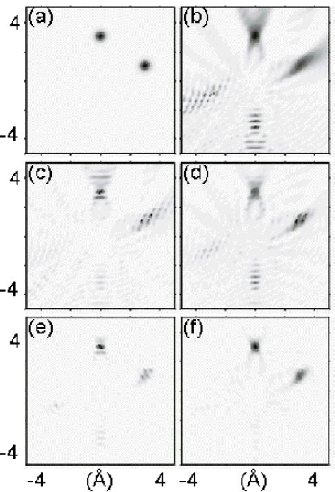
Figure 1: real space image of (a) the original charge density distribution - ${\rm{\bf F}}_{0}=50$, (b) Barton reconstruction - ${\rm{\bf F}}=400$, (c) Maximum Likelihood - ${\rm{\bf F}}=550$, (d) Maximum Entropy and - ${\rm{\bf F}}=300$, (e) constrained ML - ${\rm{\bf F}}=60$, (f) Constrained ML - ${\rm{\bf F}}=60$. (b-e) were obtained from the hologram at 17 keV in Fig. (2a) while (f) was obtained from the simulated holograms at 17 and 18 keV shown in Fig. (2a,b). The colormaps are scaled for each picture.

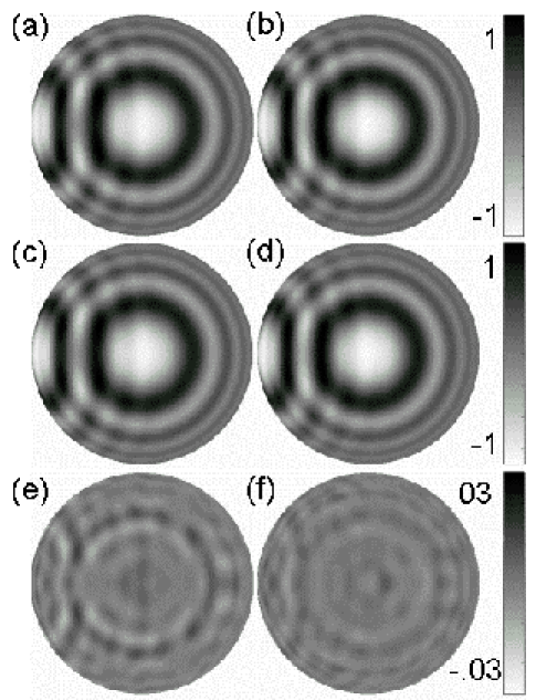
Figure 2: Top–Simulated holograms from two Gaussian charge distributions as shown in Fig. (1a) at 17 keV and (1b) 18 keV after smoothing. Center– Holograms generated by the fitted charge density distribution at the same energies (1c) 17 keV and (1d) 18 keV. Bottom– Difference between top and center: 1e = 1a - 1c and 1f = 1b - 1d.

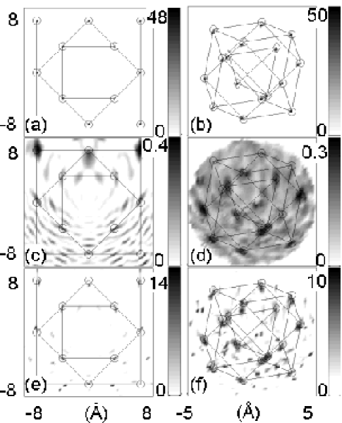
Figure 3: Top- Original charge distribution (${\rm{\bf F}}_{0}=1.8\times\;10^{4}$) - (a) XZ plane, and (b) 3D view. Center- Standard holographic reconstruction (${\rm{\bf F}}=7\times\;10^{4}$), (c) and (d) the same views as (a) and (b), respectively. Bottom–Deconvolved charge density distribution (${\rm{\bf F}}=2.9\times\;10^{4}$), (e) and (f) show the same views as (a) and (b). The colorbar shows the maximum and minimum value. The 3D images are obtained by maximum voxel (volume-pixels) projection: the 3D matrix is rotated with respect to a plane (screen). On every pixel of the screen we project the maximum value of the voxels on top of the pixel itself.

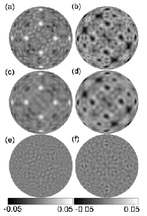
Figure 4: Top–Simulated holograms from a cluster of 1000 atoms at (a) 8 keV and (b) 9 keV after smoothing. Center– Holograms generated by the fitted charge density distribution at the same energies (a) 8 keV and (b) 9 keV. Bottom– Difference between top and center: e = a - c and f = b - d

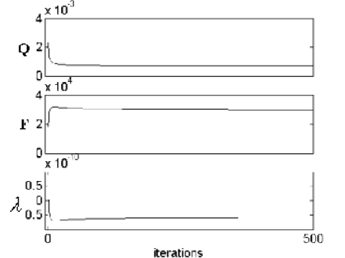
Figure 5: behavior of the fit quality (${\rm{\bf Q}}$) normalized to the volume in k-space, the number of electrons (${\rm{\bf F}}$) and the Lagrange multiplier $\lambda$. The fit is obtained quickly, while ${\rm{\bf F}}$ decreases much more slowly. The multiplier follows the behavior of ${\rm{\bf F}}$ as it tries to bring it back to ${\rm{\bf F}}_{0}\simeq 10^{4}$.

We have initially tried all the above mentioned deconvolution methods on a test system consisting of a charge distribution described by a 3D matrix of $50^{3}$ points with 0.2 Å spacing. This matrix was set to 0 except for two Gaussian charge distributions centered in the x-z plane representing two atoms separated by 3.5 Å as shown in Fig. (1a). Figures (1b-d) now show reconstructed images via several different methods obtained from a hologram (Fig. 2a) defined at an energy of 17 keV with the points distributed over a solid angle with azimuth varying from $0^{0}$ to $360^{0}$ and polar angle from $0^{0}$ (parallel to the z-axis) to $80^{0}$. The reconstruction in Fig. (1f) has been obtained using both holograms at 17 keV and 18 keV (Fig. 2b). The standard direct Barton method in Fig. (1b) shows a weak twin image, and some distortion of the imaged charge distributions, with the difference between Fig. (1a) and Fig. (1b) essentially being the PSF. The number of electrons estimated from the Barton method is one order of magnitude bigger than the original one. This could be ascribed to the fact that many of these electrons are not contributing to the hologram, as they cancel each other. In trials with the Van Cittert and ML (Fig. 1c) methods using the double pixel approximation, we have found that the convergence is very good: less then 10 iterations are necessary for convergence. This is due to the fact that the holographic reconstruction is a relatively good image of the charge density. However the number of electrons used to fit the data was one order of magnitude bigger than that of the original image. Another relevant feature of this method is the fact that the image becomes more structured. This is due to the divergence in the inverse of the Hessian using single energy holograms when ${\rm{\bf H}}_{{\rm{\bf r}},{\rm{\bf r}}}={\rm{\bf H}}_{{\rm{\bf r}},-{\rm{\bf r}}}$.

Tests using the Lucy-Richardson method have shown bad convergence; further studies of this method need to be done, but one of the reasons could be some divergence caused by the denominator in equation (6).

At this point we turned to the maximum entropy method. As we had already developed the ML algorithm with single and double pixel approximations, we could easily apply the algorithm developed by Cornwell and Evans Cornwell:1985 so as to employ the maximum entropy criterion. This algorithm tries to maximize the entropy ${\rm{\bf S}}$ while minimizing the likelihood ${\rm{\bf Q}}$ with a fixed number of electrons ${\rm{\bf F}}$ using Lagrange multipliers. Several tests have shown that this algorithm (at least the one implemented by us) was not able to minimize ${\rm{\bf Q}}$, ${\rm{\bf S}}$ and ${\rm{\bf F}}$ at the same time; the result is shown in Fig. (1d). However, we did find that the maximum likelihood and the minimum number of electrons produces a good quality reconstruction, with somewhat improved resolution, and a reasonably good ${\rm{\bf F}}$Marchesini:2001 ; these results are shown in Fig. (1e) and they can be compared with those in (1b). The number of electrons is only 20% bigger than the original one.

The single energy iterative reconstruction shows how the divergence in the Hessian due to the twin image problem produces several artifacts, which are removed when using slightly different energies (Fig. 1f). The reason why the number of electrons does not correspond to the original ${\rm{\bf F}}_{0}$ even when applying the constraint is that after the steps are applied, we impose positivity by setting to 0 the negative values of the density.

Finally, we applied the constrained ML method to the same case, using a double-energy data set. This result is shown in Fig. (1f) and represents the most significant enhancement in image quality relative to the standard method.

To explore the constrained ML algorithm further, we carried out simulations based on a much larger and more realistic cluster of atoms representing CdTe; the charge density distribution in the neighborhood of the origin is shown in Fig. (3a,b). We tried to keep a minimum amount of information to show the robustness of the method: We simulated the hologram produced by a CdTe cluster of 1000 atoms at only two energies of 8 and 9 keV. At these two energies the holographic reconstruction using the Barton method shows a poor image quality as shown in Fig. (3c,d). We also introduced a randomly distributed noise level of $10^{-3}$ on every data point (corresponding to 10⁶ counts in each point), with the points distributed over a solid angle with azimuth varying from 0 to 360 degrees and polar angle from 0 (perpendicular to the [001] surface normal direction) to 80 degrees, with a 1-degree step size in each direction. Since we are interested in imaging the first neighbors, we finally carried out all imaging with a smoothed hologram based on 2 degree smoothing in every direction. Although the cluster size is several nanometers, we will only try to reconstruct up to 8 Å setting to 0 anything outside this range.

The holograms generated by this charge after smoothing are shown in Fig. (4a) at 8 keV and Fig. (4b) at 9 keV. We again choose as a first reference step and set of images the standard holographic reconstruction in Fig. (3a,b). Comparison between the standard reconstruction and the deconvolved images are shown in Fig. (3c,f).

The number of electrons within the reconstructed region is ${\rm{\bf F}}_{0}=1.8\times\;10^{4}$ in the original picture, ${\rm{\bf F}}=7\;\times 10^{4}$ in the standard reconstruction, and ${\rm{\bf F}}=2.9\times\;10^{4}$ in the deconvolved image. Thus, the deconvolved image is a factor of 1.5 larger than the original image in number of electrons, but a factor of 2 better than the standard reconstruction. This result is worse than what we observed for the two Gaussian charges, and can be ascribed to the difficulty to fit point like structures (atoms) at the diffraction limit scale instead of smooth distributions. The peak heights of the charge density in the three images varies somewhat differently, the maximum number of electrons in one voxel in the original image is 50, 0.38 in the standard reconstruction, and 14 in the deconvolved image, as shown more quantitatively in the colorbars of Fig. (3). The reason for this is that in the original image, every electron of one atom is concentrated in a single voxel, while the standard reconstruction has many electrons spread over many more voxels. The deconvolved image has a total of fewer electrons than the standard image, but much higher peaks, due to the enhanced resolution relative to the standard reconstruction. Comparing image quality between the standard (Fig. 3c,d) and deconvolved (Fig. 3e,f) approaches, we see a definite enhancement of resolution in the deconvolved images, even though some artifacts remain that are of comparable strength to the actual charge-density images. The holograms generated by the cluster in Fig. (4a,b) are well described in the low frequency range by the fitted holograms in Fig. (4c) (8 keV) and Fig. (4d). Since in the iterations we only fitted the charge density within the first 8 Å setting the distribution to 0 outside this range, only the low frequency components where fitted, as the residual difference shows in Fig. (4e-f).

In Fig. (5), we present some results dealing with the rapidity and type of convergence observed. The maximum likelihood is obtained within the first 10-20 iterations (Fig. 5-top). The total number of electrons is slowly reduced in the following $\sim 500$ iterations (Fig. 5-center). The Lagrange multiplier $\lambda$ follows the behavior of the constraint: as ${\rm{\bf F}}$ changes from the desired level ${\rm{\bf F}}_{0}$, $\lambda$ varies in order to bring ${\rm{\bf F}}$ back to the desired level.

VI Conclusions and future possibilities

In conclusion, we have demonstrated that iterative deconvolution can be applied to XFH imaging, thus improving the quality of the images beyond the diffraction limit, and that several levels of approximation can be used. From our test cases, the constrained maximum likelihood method appears to be the most promising. In these first theoretical simulations related to image improvement, we have approximated the scattering factor as isotropic, thus neglecting the angular dependence of Thomson scattering and near-field effects. As a computationally relevant issue, we have also approximated the Hessian to be a sparse matrix where only the two diagonals are non-zero. All of these approximations could be relaxed in future applications, including terms close to the diagonals, with of course additional complexity then being incurred in the deconvolution algorithm and the length of time it takes. For our calculations, the storage and calculation of the full Hessian of $80^{6}$ points required considerable memory, but computers capable of such calculations should be available as desktops in a few years. The gradient was also calculated neglecting the angular dependence of the scattering factor. Using these approximations, every iteration involved the calculation of a hologram from a matrix of $80^{3}$ voxels, the reconstruction and required about 5 minutes on a Pentium II computer, for a total of one night of calculation. Our image deconvolution has been obtained by enforcing a real and positive charge density distribution and limited number of electrons. However, looking ahead to further image improvement, once the image is deconvolved, one could make use of ‘atomicity’ in the next step by placing atoms in the location of the peaks, and then performing an optimization using the full angular dependence of the scattering factor, while simultaneously adjusting the atomic number and position of these atoms. This study thus suggests several fruitful directions for further exploration and exploitation of image deconvolution in x-ray fluorescence holography that should considerably enhance its power for structural studies.

Appendix A Appendix–Calculation of the Hessian and the gradient

The Hessian does not need to be known in great detail. It can be pre-calculated before starting the iterative algorithm neglecting the angular dependence of Thompson scattering factor $\frac{f_{T}}{r_{e}}=\frac{1+\cos^{2}\Theta_{{\rm{\bf k}},{\rm{\bf r}}}}{2}$ and using the following approximation $\int\limits_{\sigma\left(k\right)}{\cos^{2}\left({kr-{\rm{\bf k}}\cdot{\rm{\bf r}}}\right)\,k^{2}d^{2}{\rm{\bf\hat{k}}}}\simeq\textstyle{1\over 2}\Omega_{k}$ and $\int\limits_{\sigma\left(k\right)}{\sin^{2}\left({{\rm{\bf k}}\cdot{\rm{\bf r}}}\right)\,k^{2}d^{2}{\rm{\bf\hat{k}}}}\simeq\textstyle{1\over 2}\Omega_{k}$, with $\Omega_{k}=\int_{\sigma\left(k\right)}{k^{2}d^{2}{\rm{\bf\hat{k}}}}$, ${\rm{\bf\hat{k}}}$ is a unit vector, and $\sigma(k)$ is the region where the hologram is measured at a given energy. This yields:

$${\rm{\bf H}}_{{\rm{\bf r}},{\rm{\bf r}}} = \sum\nolimits_{k}{\Delta k\int_{\sigma(k)}{\textstyle{{r^{2}}\over{r_{e}^{2}}}\cos^{2}\left({kr-{\rm{\bf k}}\cdot{\rm{\bf r}}}\right)\,k^{2}d^{2}{\rm{\bf\hat{k}}}}},$$

$$\simeq \textstyle{{r^{2}}\over{r_{e}^{2}}}\textstyle{1\over 2}\sum\nolimits_{k}{\Omega_{k}\,\Delta k}\,;$$

$${\rm{\bf H}}_{{\rm{\bf r}},-{\rm{\bf r}}} = \sum\nolimits_{k}{\Delta k\int_{\sigma(k)}{\textstyle{r\over{r_{e}}}\cos\left({kr-{\rm{\bf k}}\cdot{\rm{\bf r}}}\right)}}$$ (20)

$$\times\cos\left({kr+{\rm{\bf k}}\cdot{\rm{\bf r}}}\right)\,k^{2}d^{2}\hat{k}$$

$$= \textstyle{{r^{2}}\over{r_{e}^{2}}}\sum\nolimits_{k}{\Delta k\int_{\sigma(k)}{\left[{\cos^{2}\left({kr}\right)-\sin^{2}\left({{\rm{\bf k}}\cdot{\rm{\bf r}}}\right)}\right]k^{2}d^{2}{\rm{\bf\hat{k}}}}},$$

$$\simeq \textstyle{{r^{2}}\over{r_{e}^{2}}}\sum\nolimits_{k}{\left[{\cos^{2}\left({kr}\right)-\textstyle{1\over 2}}\right]\Omega_{k}\,\Delta k}$$

$$\simeq \textstyle{1\over 2}\textstyle{{r^{2}}\over{r_{e}^{2}}}\sum\nolimits_{k}{\cos\left({2kr}\right)\Omega_{k}\,\Delta k}\;;$$

The gradient is calculated by simulating the hologram $\chi^{\left\{n\right\}}\left({\rm{\bf k}}\right)$ generated by a charge density distribution $\rho^{\left\{n\right\}}\left({\rm{\bf r}}\right)$, and propagating back the hologram to the real space. Using $\bar{U}\left({\rm{\bf r}}\right)=\left({\textstyle{r\over{r_{e}}}}\right)^{2}U\left({\rm{\bf r}}\right)$, eq. (8) can be written as:

$$\nabla{\rm{\bf Q}} = 2\left[{\bar{U}^{\left\{n\right\}}\left({\rm{\bf r}}\right)-\bar{U}\left({\rm{\bf r}}\right)}\right];$$

$$\bar{U}^{\left\{n\right\}}\left({\rm{\bf r}}\right) = \eta^{\dagger}\left({{\rm{\bf r}},{\rm{\bf k}}}\right)\cdot\chi^{\left\{n\right\}}\left({\rm{\bf k}}\right)$$

$$\simeq \frac{2r}{\Omega r_{e}}{\rm Re}\int_{\sigma}{e^{-i\left({kr-{\rm{\bf k}}\cdot{\rm{\bf r}}}\right)}\chi^{\left\{n\right\}}\left({\rm{\bf k}}\right)d^{3}{\rm{\bf k}}};$$

$$\chi^{\left\{n\right\}}\left({\rm{\bf k}}\right) = \eta\left({{\rm{\bf k}},{\rm{\bf r}}}\right)\cdot\rho^{\left\{n\right\}}\left({\rm{\bf r}}\right)$$ (21)

$$\simeq 2{\rm Re}\int{\textstyle{r\over{r_{e}}}e^{i\left({kr-{\rm{\bf k}}\cdot{\rm{\bf r}}}\right)}\rho^{\left\{n\right\}}\left({\rm{\bf r}}\right)d^{3}{\rm{\bf r}}}\,.$$

These calculations can be very long as we need to sum over ${\rm{\bf r}}(x,y,z)$ for every ${\rm{\bf k}}\left({k,\vartheta,\varphi}\right)$. Supposing that the number of points in $x,y,z,\vartheta,\varphi$ is $N\sim 100$ for every variable, we need to calculate the product in the integral of eq. (21) for every possible value, i.e. $N^{5}$ products and sums. The computation of $\chi^{\left\{n\right\}}\left({\rm{\bf k}}\right)$ can be performed faster if we separate the sum over the variables $x,y,z$.

We begin by calculating $\xi^{\{n\}}\left({\rm{\bf r}}\right)=\textstyle{r\over{r_{e}}}e^{ikr}\rho^{\left\{n\right\}}\left({\rm{\bf r}}\right)\Delta r^{3}$; we can express Eq. (21) as:

$$\chi_{n}\left({\rm{\bf k}}\right)\simeq 2{\rm Re}\sum_{{\rm{\bf r}}}{e^{i{\rm{\bf k}}\cdot{\rm{\bf r}}}\xi^{\{n\}}\left({\rm{\bf r}}\right)}$$ (22)

which is a simple Fourier transform. However the holograms are usually measured in spherical coordinates, and to obtain the values of $\chi_{n}\left({\rm{\bf k}}\right)$ in the measured positions, we either need to perform an interpolation, or a convolution. Another approach is to use directly the spherical coordinates in the kernel:

$$e^{i{\rm{\bf k}}\cdot{\rm{\bf r}}} = e^{ikx\sin\vartheta\cos\varphi}e^{iky\sin\vartheta\sin\varphi}e^{ikz\cos\vartheta}$$ (23)

$$= A_{k,x,\vartheta,\varphi}B_{k,y,\vartheta,\varphi}C_{k,z,\vartheta}$$

and Eq. (22) becomes:

$$\chi^{\{n\}}\left({k,\vartheta,\varphi}\right) \simeq 2{\rm Re}\sum\nolimits_{x}{A_{k,x,\vartheta,\varphi}\sum\nolimits_{y}{B_{k,y,\vartheta,\varphi}}}$$ (24)

$$\times\sum\nolimits_{z}{C_{k,z,\vartheta}\,\xi^{\{n\}}\left({x,y,z}\right)}\,.$$

Each sum requires $N^{4}$ calculation, reducing the time to perform the calculation by $\sim$N/3. The same trick can be applied for the holographic reconstruction.

References

- (1) A. Szöke, AIP Conf. Proc. 147, 361 (ed. by D.T. Attwood and J. Boker, AIP, New York, NY, 1986).
- (2) M. Tegze, G. Faigel, Nature 380, 49 (1996).
- (3) T. Gog et al. Phys. Rev. Lett. 76, 3132 (1996).
- (4) R. Fitzgerald, Physics Today 54, 21-3 (2000).
- (5) K. Hayashi et al., Anal. Sci. 14, 987 (1998).
- (6) M. Tegze, G. Faigel, S. Marchesini, M. Belakhovsky, O. Ulrich, Nature 407, 38 (2000).
- (7) S. Marchesini, F. Schmithüsen, M. Tegze, G. Faigel, Y. Calvayrac, M. Belakhovsky, J. Chevrier, A. S. Simionovici, Phys. Rev. Lett. 85, 4723 (2000).
- (8) M. Tegze, G. Faigel, S. Marchesini, M. Belakhovsky, Phys. Rev. Let. 82, 4847 (1999)
- (9) H. Stark Image Recovery: Theory and Application, Academic Press, (1987)
- (10) P. H. Van Cittert, Z. Physik 69, 298 (1931). For a more modern and English reference see e. g. P. A. Jansson, Journ. Opt. Soc. Am. 60, 184-191 (1970).
- (11) L. B. Lucy, Astronomical Journal 79, (1974), 745-54
- (12) W. H. Richardson, JOSA 62, (1972), 55-59
- (13) W. H. Press, S. A. Teukolsky, W. T. Vetterling, B. P. Flannery, Numerical Recipes in C, Cambridge University Press, (1992).
- (14) G. Faigel, M. Tegze, Reports on Progress in Physics 62, 355 (1999).
- (15) J. J. Barton, Phys. Rev. Lett. 61, 1356 (1988).
- (16) B. P. Tonner, Z.-L. Han, G. R. Harp, and D. K. Saldin, Phys. Rev. B 43, 14423 (1991).
- (17) J. Miao et al., Nature (London) 400, 342 (1999).
- (18) R. W. Gerchberg, W. O. Saxton, Optik 35, 237 (1972).
- (19) J. Fienup, Appl. Opt. 21, 2758 (1982).
- (20) S. W. Wilkins, J. N. Varghese and M. S. Lehmann, Acta Cryst A39, 47-60 (1983)
- (21) T. J Cornwell, K. F. Evans, Astronomy and Astrophysics 143, 77-83 (1985),
- (22) A. Szöke, Acta Cryst. A49, 853-866 (1993),.
- (23) S. Marchesini, C. S. Fadley, M. R. Howells, presented at “New Approaches to the Phase Problem for Non-Periodic Objects”, May 17-19, 2001, Lawrence Berkeley National Laboratory, available at www-esg.lbl.gov/esg/meetings/phasing/