Holographic analysis of diffraction structure factors

Abstract

We combine the theory of inside-source/inside-detector x-ray fluorescence holography and Kossel lines/x ray standing waves in kinematic approximation to directly obtain the phases of the diffraction structure factors. The influence of Kossel lines and standing waves on holography is also discussed. We obtain partial phase determination from experimental data obtaining the sign of the real part of the structure factor for several reciprocal lattice vectors of a vanadium crystal.

The phase determination of diffracted beams is the central problem of x-ray crystallography. Several methods exist to obtain this information, such as direct methods Sayre:1995 , 3-beam diffraction Shen:1987 , anomalous diffraction, heavy atom or molecular replacement Blundell:1976 and x-ray standing waves or Kossel lines von:1960 ; Batterman:1964 ; Cowley:1964 . Despite the many advances in these methods, not all problems can be solved. Direct methods fail when the unit cell contains a large number of atoms. Anomalous diffraction and related methods are among the most successful methods for biological crystallography, but they often require chemical modification of the molecules. Multiple beam diffraction, x-ray standing waves and Kossel lines have usually been applied only to high-quality crystals of relatively simple structures, or to the localization of dopants in high quality crystals Golovchenko:1974 .

Kossel lines are formed when a source of short wavelength radiation ($\sim 1$ Å) is located on a crystallographic site: they result from the Bragg scattering of outgoing fluorescent x-rays from various sets of planes in the lattice. In the notation of holography, this is an “inside-source” experiment. The fine structure of these lines has been explained by the dynamical theory of x-ray diffraction via the reciprocity theorem used in optics von:1960 . A proper analysis of the KL fine structure allows the determination of the phases of reflections Batterman:1964 ; Cowley:1964 ; Gog:1995 ; Vartanyants:2001 ; Lonsdale:1949 . In parallel to this work on KL, the x-ray standing wave (XSW) method has been developed Batterman:1964 ; Cowley:1964 ; Golovchenko:1974 ; Vartanyants:2001 . In this case, the source and the detector are interchanged as compared to the KL method: the atoms are subject to the changing wave-field in the crystal as the incident beam goes through a Bragg reflection, and fluorescent radiation proportional to the field at the atom is generated. This constitutes the ”inside-detector” configuration in holography Gog:1995 . Besides the fine structure of the KL or XSW produced when the crystal orientation satisfies a Bragg or Laue condition, tails are formed far from the Bragg angle. These coarse features, also formed by poorer-quality mosaic crystals provide information on the real and imaginary part of the structure factor Vartanyants:2001 ; Lonsdale:1949 .

Unlike standard imaging methods, holography offers the possibility of extracting both intensity and phase information. X-ray fluorescence holography (XFH) is thus a very promising new method for obtaining a direct image in real space of the local environments of different atomic species in reasonably well-ordered crystals or molecular ensembles. Long-range translational order is not required, and indeed one of the most important results obtained by XFH has been the imaging of the average local environment of a quasicrystal Marchesini:2000 . Despite this, with the exception of quasicrystals, all systems measured so far have been well-ordered crystals Tegze:1999 ; Hiort:2000 ; Tegze:2000 ; Kopecky:2001 .

In this paper we develop a theoretical method for analyzing the inside-source and inside-detector holograms of a periodic object using the kinematic approximation. By analyzing the holographic reconstruction in reciprocal space, we discuss how to obtain directly the phase of the structure factors. We also show how the standard holographic analysis is affected by diffraction, and discuss the solution to this problem.

A hologram is formed whenever an unknown object wave $E_{obj}$ is coherently added to a reference wave $E_{ref}$:

$$I\left(\bm{\mathrm{k}}\right) = \left|{E_{\text{ref}}+E_{\text{obj}}}\right|^{2}$$ (1)

$$= I_{\text{ref}}+I_{\text{obj}}+2\mathrm{Re}\left\{{E_{\text{ref}}^{\ast}E_{\text{obj}}}\right\}.$$

where $I_{ref}$ and $I_{obj}$ are the intensities of the reference and object waves respectively.

The hologram is extracted by subtracting the reference beam intensity $I_{ref}$ and normalizing. The object term $I_{obj}$ is usually assumed to be small and therefore neglected in order to permit a holographic analysis of the data in XFH. We will see later how this approximation can affect our analysis. When an atom located at the origin emits (inside source) or detects (inside detector) radiation, the resulting hologram (considering only the last term in eq. (1), i.e. the interference term) can be expressed as Hiort:2000 :

$$\chi\left(\bm{\mathrm{k}}\right)=-2\mathrm{Re}\sum\limits_{\bm{\mathrm{r}}}{f(\bm{\mathrm{k}},\bm{\mathrm{r}})\,}\,\chi_{\bm{\mathrm{r}}}\left(\bm{\mathrm{k}}\right),$$ (2)

where $\chi_{\bm{\mathrm{r}}}\left(\bm{\mathrm{k}}\right)\equiv\,-\textstyle{{e^{i\left({kr-\bm{\mathrm{k}}\cdot\bm{\mathrm{r}}}\right)}}\over r}$ and $f(\bm{\mathrm{k}},\bm{\mathrm{r}})$ is the scattering factor (including the Thompson scattering factor Len:1997 ) of the atom located at $\bm{\mathrm{r}}$. The summation is extended to all the atomic positions.

Ideally, when the object term can be neglected and the scattering factors are isotropic, the holograms $\chi_{\bm{\mathrm{r}}}\left(\bm{\mathrm{k}}\right)$, $\quad\chi_{{\bm{\mathrm{r}}}^{\prime}}\left(\bm{\mathrm{k}}\right)$ generated by two point scatterers located at $\bm{\mathrm{r}}$ and ${\bm{\mathrm{r}}}^{\prime}$, are orthogonal. i.e. $\quad\left\langle{\chi_{\bm{\mathrm{r}}}^{\ast}\left(\bm{\mathrm{k}}\right)\,\chi_{{\bm{\mathrm{r}}}^{\prime}}\left(\bm{\mathrm{k}}\right)}\right\rangle_{\bm{\mathrm{k}}}\simeq$$\alpha\left(\bm{\mathrm{r}}\right)\delta\left({\bm{\mathrm{r}}-{\bm{\mathrm{r}}}^{\prime}}\right)$. $\alpha\left(\bm{\mathrm{r}}\right)$ is a normalization function and $\left\langle\right\rangle_{\bm{\mathrm{k}}}$ is the average on the measured k space. The two holograms are orthogonal because the relative phase oscillates when the infinite k-space is spanned. In normal situations, due in particular to the limited k-space sampling, $\delta\left({\bm{\mathrm{r}}-{\bm{\mathrm{r}}}^{\prime}}\right)$ becomes a point spread function peaked in $\bm{\mathrm{r}}={\bm{\mathrm{r}}}^{\prime}$. The typical reconstruction algorithm is based on this orthogonality assumption. The holographic reconstruction is the projection of $\chi\left(\bm{\mathrm{k}}\right)$ onto $\chi_{{\bm{\mathrm{r}}}^{\prime}}\left(\bm{\mathrm{k}}\right)$:

$$U\left({\bm{\mathrm{r}}}^{\prime}\right)=\left\langle{\chi\left(\bm{\mathrm{k}}\right)\chi_{{\bm{\mathrm{r}}}^{\prime}}^{*}\left(\bm{\mathrm{k}}\right)}\right\rangle_{\bm{\mathrm{k}}}\,.$$ (3)

What happens if we now perform the reconstruction taking into account the long-range periodicity of the system? To answer this question, let us first examine the holographic reconstruction in the reciprocal space, by applying a Fourier transform to eq. (3). Since only the kernel $\chi_{{\bm{\mathrm{r}}}^{\prime}}\left(\bm{\mathrm{k}}\right)$ depends on ${\bm{\mathrm{r}}}^{\prime}$ we can bring the FT inside the average and write:

$$G({\bm{\mathrm{h}}}^{\prime}) = \left\langle{\chi\left(\bm{\mathrm{k}}\right)\int{d^{3}\bm{\mathrm{r}}\,e^{i{\bm{\mathrm{h}}}^{\prime}\cdot\bm{\mathrm{r}}}\,}\chi^{*}_{\bm{\mathrm{r}}}\left(\bm{\mathrm{k}}\right)}\right\rangle_{\bm{\mathrm{k}}}$$

$$= \left\langle{\chi\left(\bm{\mathrm{k}}\right)\tilde{\chi}^{*}_{{\bm{\mathrm{h}}}^{\prime}}\left(\bm{\mathrm{k}}\right)}\right\rangle_{\bm{\mathrm{k}}}\;,$$

$$\tilde{\chi}_{\bm{\mathrm{h}}}\left(\bm{\mathrm{k}}\right) = \int{d^{3}\bm{\mathrm{r}}\textstyle{{-1}\over r}e^{i\left\{{kr-(\bm{\mathrm{k}}-\bm{\mathrm{h}})\cdot\bm{\mathrm{r}}}\right\}}\,}=\textstyle{{-1}\over{\left({\left|{\bm{\mathrm{k}}-\bm{\mathrm{h}}}\right|^{2}-k^{2}}\right)}}\;.$$ (5)

The formal analogy between (3) and (Holographic analysis of diffraction structure factors) suggests we consider $\tilde{\chi}_{\bm{\mathrm{h}}}\left(\bm{\mathrm{k}}\right)$ as the hologram generated by a point structure factor, located at position $\bm{\mathrm{h}}$ of the reciprocal space, $i.e.$ a sinusoidal charge density distribution with unitary scattering factor amplitude. Similarly to the discussion above, we expect the holograms $\tilde{\chi}_{{\bm{\mathrm{h}}}^{\prime}}\left(\bm{\mathrm{k}}\right),\;\tilde{\chi}_{\bm{\mathrm{h}}}\left(\bm{\mathrm{k}}\right)$ generated by two points $\bm{\mathrm{h}}$ and ${\bm{\mathrm{h}}}^{\prime}$ in the reciprocal lattice to be orthogonal in k-space, $i.e.\quad\left\langle{\tilde{\chi}_{{\bm{\mathrm{h}}}^{\prime}}^{\ast}\left(\bm{\mathrm{k}}\right)\tilde{\chi}^{*}_{\bm{\mathrm{h}}}\left(\bm{\mathrm{k}}\right)}\right\rangle\simeq\beta\left(\bm{\mathrm{h}}\right)\delta\left({\bm{\mathrm{h}}-{\bm{\mathrm{h}}}^{\prime}}\right)$. In real situations the Dirac delta function is replaced by a function peaked in $\bm{\mathrm{h}}$.

We now examine the properties of the hologram $\chi\left(\bm{\mathrm{k}}\right)$ in terms of the structure factors of the reciprocal lattice vectors. Following Adams:1998 , we rewrite (2) in terms of the electron density $\rho\left(\bm{\mathrm{r}}\right)$:

$$\chi\left(\bm{\mathrm{k}}\right)=2\mathrm{Re}\int{d^{3}\bm{\mathrm{x}}\,\rho(\bm{\mathrm{r}})}\,\,\textstyle{{-r_{e}}\over r}e^{i(kr-\bm{\mathrm{k}}\cdot\bm{\mathrm{r}})}\;,$$ (6)

where $r_{e}$ is the classical electron radius. For simplicity we have approximated the Thompson scattering factor to be a constant. If the system is periodic, the charge density distribution can be expressed in a Fourier series in terms of the reciprocal lattice vectors $\bm{\mathrm{h}}$ and the relative structure factors $F_{\bm{\mathrm{h}}}$, namely $-r_{e}\rho\left(\bm{\mathrm{r}}\right)=\sum\nolimits_{\bm{\mathrm{h}}}{F_{\bm{\mathrm{h}}}}e^{i\bm{\mathrm{h}}\cdot\bm{\mathrm{r}}}$, with $F_{\bm{\mathrm{h}}}=\textstyle{{-r_{e}}\over V}\int\limits_{V}{\rho\left(\bm{\mathrm{r}}\right)\;e^{i\bm{\mathrm{h}}\cdot\bm{\mathrm{r}}}d}^{3}\bm{\mathrm{r}}$, where $V$ is the unit cell volume. The origin, which determines the phase shifts in the structure factors, is at the emitting atom in the unit cell.

The hologram (6) becomes, in analogy with (2):

$$\chi\left(\bm{\mathrm{k}}\right)=2\mathrm{Re}\sum\limits_{\bm{\mathrm{h}}}{F_{\bm{\mathrm{h}}}\tilde{\chi}_{\bm{\mathrm{h}}}\left(\bm{\mathrm{k}}\right)\;}.$$ (7)

The divergence of $\tilde{\chi}_{\bm{\mathrm{h}}}\left(\bm{\mathrm{k}}\right)$ at the Bragg condition ($\bm{\mathrm{h}}^{2}-2\bm{\mathrm{h}}\cdot\bm{\mathrm{k}}=0)$ in (5) is introduced as a consequence of neglecting extinction, mosaicity and the finite sample size. These effects can be approximated by writing $k$ as a complex number The:1 , i.e. $k=k_{r}+ik_{i}$, and $\tilde{\chi}_{\bm{\mathrm{h}}}\left(\bm{\mathrm{k}}\right)=\mathrm{Re}\left\{{\tilde{\chi}_{\bm{\mathrm{h}}}\left(\bm{\mathrm{k}}\right)}\right\}+i\mathrm{Im}\left\{{\tilde{\chi}_{\bm{\mathrm{h}}}\left(\bm{\mathrm{k}}\right)}\right\}$ then becomes:

$$\mathrm{Re}\left\{{\tilde{\chi}_{\bm{\mathrm{h}}}\left(\bm{\mathrm{k}}\right)}\right\} = \left|{\tilde{\chi}_{\bm{\mathrm{h}}}\left(\bm{\mathrm{k}}\right)}\right|^{2}\left({\bm{\mathrm{h}}^{2}-2\bm{\mathrm{h}}\cdot\bm{\mathrm{k}}}\right),$$

$$\mathrm{Im}\left\{{\tilde{\chi}_{\bm{\mathrm{h}}}\left(\bm{\mathrm{k}}\right)}\right\} = \left|{\tilde{\chi}_{\bm{\mathrm{h}}}\left(\bm{\mathrm{k}}\right)}\right|^{2}\left({-2k_{i}k_{r}}\right),$$

$$\left|{\tilde{\chi}_{\bm{\mathrm{h}}}\left(\bm{\mathrm{k}}\right)}\right|^{2} = \textstyle{1\over{\left({\bm{\mathrm{h}}^{2}-2\bm{\mathrm{h}}\cdot\bm{\mathrm{k}}}\right)^{2}+\left({2k_{i}k_{r}}\right)^{2}}}\;.$$ (8)

As the wave-vector $\bm{\mathrm{k}}$ changes across the pole of $\tilde{\chi}_{\bm{\mathrm{h}}}\left(\bm{\mathrm{k}}\right)$, there will be a symmetric and an antisymmetric contribution dependent in different ways on the real and the imaginary part of the structure factor. Writing $F_{\bm{\mathrm{h}}}=\mathrm{Re}\left\{{F_{\bm{\mathrm{h}}}}\right\}+i\,\mathrm{Im}\left\{{F_{\bm{\mathrm{h}}}}\right\}$, the hologram in (7) becomes:

$$\chi=2\sum\limits_{\bm{\mathrm{h}}}{\mathrm{Re}\left\{{\tilde{\chi}_{\bm{\mathrm{h}}}}\right\}\mathrm{Re}\left\{{F_{\bm{\mathrm{h}}}}\right\}}-\mathrm{Im}\left\{{\tilde{\chi}_{\bm{\mathrm{h}}}}\right\}\mathrm{Im}\left\{{F_{\bm{\mathrm{h}}}}\right\}\,.$$ (9)

Note that, at the Bragg condition, the object term cannot be neglected, it contributes with a second order divergence and therefore needs to be added to the interference term. The normalized object term can then be written as:

$$\frac{I_{obj}}{I_{ref}}=\sum\limits_{\bm{\mathrm{h}}}{\left|{F_{\bm{\mathrm{h}}}}\right|^{2}\left|{\tilde{\chi}_{\bm{\mathrm{h}}}}\right|}^{2}+\sum\limits_{\bm{\mathrm{h}},{\bm{\mathrm{h}}}^{\prime}\neq\bm{\mathrm{h}}}{F_{\bm{\mathrm{h}}}^{\ast}F_{{\bm{\mathrm{h}}}^{\prime}}\tilde{\chi}_{\bm{\mathrm{h}}}^{\ast}\tilde{\chi}_{{\bm{\mathrm{h}}}^{\prime}}}\;.$$ (10)

Except when multiple Bragg conditions are satisfied simultaneously, the second term can be neglected. We recall that the object wave intensity is always smaller than that of the reference at a pole $\textstyle{{I_{obj}}\over{I_{ref}}}\approx\left|{\textstyle{{F_{\bm{\mathrm{h}}}}\over{\left({2k_{r}k_{i}}\right)}}}\right|^{2}<1$, while the interference term (9), at a Bragg condition, is $\textstyle{{\mathrm{Im}F_{\bm{\mathrm{h}}}}\over{k_{r}k_{i}}}$. The interference term (9) can still be the dominant one, depending on the phase of the structure factor.

Let us now consider the properties of the reconstructed image $G$, which can be viewed as the ‘hologram of the reciprocal lattice’, in relation to the structure factors. The real and imaginary parts of the reconstruction kernel $\tilde{\chi}_{{\bm{\mathrm{h}}}^{\prime}}\left(\bm{\mathrm{k}}\right)$ (eq. (8)) are respectively antisymmetric and symmetric across the pole as $\left({{\bm{\mathrm{h}}}^{\prime 2}-2{\bm{\mathrm{h}}}^{\prime}\cdot\bm{\mathrm{k}}}\right)$ changes from positive to negative. The product between an antisymmetric and a symmetric function is antisymmetric, and the integral across the pole cancels out:

$$\left\langle{\mathrm{Re}\left\{{\tilde{\chi}_{\bm{\mathrm{h}}}\left(\bm{\mathrm{k}}\right)}\right\}\mathrm{Re}\left\{{\tilde{\chi}^{*}_{\bm{\mathrm{h}}}\left(\bm{\mathrm{k}}\right)}\right\}}\right\rangle_{k} = a\left(\bm{\mathrm{h}}\right),$$

$$\left\langle{\mathrm{Re}\left\{{\tilde{\chi}_{\bm{\mathrm{h}}}\left(\bm{\mathrm{k}}\right)}\right\}\mathrm{Im}\left\{{\tilde{\chi}^{*}_{\bm{\mathrm{h}}}\left(\bm{\mathrm{k}}\right)}\right\}}\right\rangle_{k} \approx 0,$$

$$\left\langle{\mathrm{Im}\left\{{\tilde{\chi}_{\bm{\mathrm{h}}}\left(\bm{\mathrm{k}}\right)}\right\}\mathrm{Im}\left\{{\tilde{\chi}^{*}_{\bm{\mathrm{h}}}\left(\bm{\mathrm{k}}\right)}\right\}}\right\rangle_{k} = -b\left(\bm{\mathrm{h}}\right);$$ (11)

where the normalization functions $a\left(\bm{\mathrm{h}}\right)$ and $b\left(\bm{\mathrm{h}}\right)$, are positive functions. The resulting holographic reconstruction becomes:

$$\mathrm{Re}\left\{{G\left({{\bm{\mathrm{h}}}^{\prime}=\bm{\mathrm{h}}}\right)}\right\} \approx {\mathrm{Re}\left\{{F_{\bm{\mathrm{h}}}}\right\}a\left(\bm{\mathrm{h}}\right)}\,,$$

$$\mathrm{Im}\left\{{G\left({{\bm{\mathrm{h}}}^{\prime}=\bm{\mathrm{h}}}\right)}\right\} \approx {\left({2\mathrm{Im}\left\{{F_{\bm{\mathrm{h}}}}\right\}-\textstyle{{\left|{F_{\bm{\mathrm{h}}}}\right|^{2}}\over{2k_{r}k_{i}}}}\right)b\left(\bm{\mathrm{h}}\right)}\;.$$

The real part of the reconstructed hologram, with ${\bm{\mathrm{h}}}^{\prime}$ equal to a reciprocal lattice vector $\bm{\mathrm{h}}$, is proportional to the real part of the structure factor. The characterization of $\mathrm{Re}\left\{{F_{\bm{\mathrm{h}}}}\right\}$ reduces the phase problem of the structure factor from the possible $(0,2\pi)$ range to only two possible values of the phase, and in the centrosymmetric systems this correspond to the complete solution. This requires us to calculate the normalization function $a\left(\bm{\mathrm{h}}\right)$, which is dependent on the measured k-space, polarization factors, extinction, sample boundaries, mosaic spread and angular resolution. Such calculation goes beyond the scope of this work; however the knowledge of the sign of $\mathrm{Re}F_{\bm{\mathrm{h}}}$ reduces the range of the possible phases by half. The imaginary part of $G$ depends on the real and imaginary part of the structure factors. If the object term $I_{obj}$ in (1) cannot be neglected, the Fourier transform of $G,$ the “standard holographic reconstruction”, would have the wrong interpretation. It would be more some kind of Patterson function (the Fourier transform of $\left|{F_{\bm{\mathrm{h}}}}\right|^{2})$ rather than a hologram (Fourier transform of $\mathrm{Re}F_{\bm{\mathrm{h}}}+i\mathrm{Im}F_{\bm{\mathrm{h}}})$. Only with the full knowledge of the normalization functions $a\left(\bm{\mathrm{h}}\right)$ and $b\left(\bm{\mathrm{h}}\right)$ can we separate and extract the values of the real and imaginary parts of the structure factors. The limitations on this straightforward analysis of the imaginary part of the structure factor apply to the standard holographic reconstruction as well. It is not surprising that a diffraction measurement interpreted as a hologram in a recent article Kopecky:2002 provides the correct structure, as the Patterson function peaks match the correct solution.

Analyzing the reconstruction in the reciprocal space allows extracting directly information on the real part of the structure factors, simplifying the problem to the calculation of the normalization functions. By including the knowledge of the absolute value of the structure factor, we can separate the contribution of the object intensity term to the imaginary part of the structure factor.

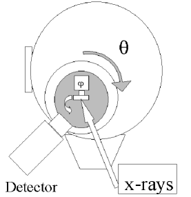
Figure 1: - Experimental setup. Monochromatic x-rays impinge on the sample, mounted on a two-axis goniometer that is rotated at high speed, and a solid-state detector collects the fluorescence radiation. Only the sample rotates, with the angle between the exciting x-rays and the detected fluorescent x-rays fixed.

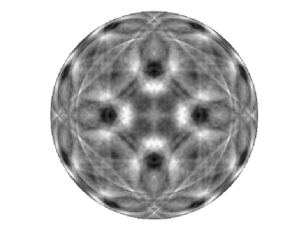
Figure 2: - Measured inside-detector hologram of a vanadium (bcc) single crystal at 4.9 keV fluorescent energy and 6.3 keV incident energy, after symmetrization and rotation of the pattern to be in the (100) orientation.

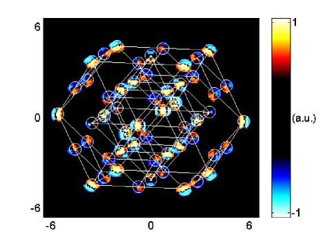
Figure 3: Reconstructed structure factor obtained from the hologram in 2; axes scale is in $2\pi/\mbox{{\AA}}$, the colorbar is in arbitrary units. Circles indicate the locations of the reciprocal vectors, with these being connected by light lines. At each circle, there is a positive peak, as expected for this system.

We performed the experiments on a bending magnet beamline (BL 9.3.1) at the Advanced Light Source. A schematic drawing of the experimental setup is shown in Figure 1. Inside the chamber, the sample, a vanadium bcc single crystal with (111) orientation, is mounted on a standard two-axis goniometer. The V $K_{\alpha}$ fluorescence radiation at 4.9 keV emitted by the sample was collected by a 4-channel high-speed solid state detector with single photon pulse analysis and a maximum of 4 MHz count rate Bucher:1996 . The measurement was performed by rotating the sample at high speed in a spiral motion Marchesini:2001 : the azimuth at 3600 degrees per second, and the polar at 2 degrees per second and varying from 0 (perpendicular to the surface) to 80 degrees. The detector was placed close to the sample to average the “inside source” hologram, resulting in an ”inside-detector” measurement in holographic terminology Gog:1996 . The azimuth stepper motor pulses were used to synchronize the data acquisition allowing us to collect a full pattern of 3.2 10⁵ pixels in about 40 seconds. The measurement was repeated until the statistical noise and incident beam fluctuations have been reduced to a reasonable level; typically, several hundred separate patterns were thus summed in a final dataset.

The measured hologram at 6.3 keV incident energy is shown in Figure 2 and the real part of the reconstructed ‘reciprocal’ hologram $\mathrm{Re}\left\{{G\left({\bm{\mathrm{h}}}^{\prime}\right)}\right\}$ as derived from Eqs. 4 and 5 is shown in Figure 3. The network of white lines connects the known positions of the reciprocal lattice positions in the V lattice. The image in reciprocal space shows its most intense yellow spots at the reciprocal lattice positions, which in turn correspond to the positive values of the real part of the structure factors. One can see that the height of these peaks is approximately constant. This is because the functions $a\left(\bm{\mathrm{h}}\right)$ and $b\left(\bm{\mathrm{h}}\right)$ are almost constant when $\left|\bm{\mathrm{h}}\right|$ is not close to the wavenumber $k$, this can be true if the hologram is measured at a single energy in every direction, as was our case. The vanadium crystal is a special case in which the structure factors are real and positive. However the reconstructed image from a simulated Kossel line pattern of a PbSe single crystal which was chosen since it exhibit both positive and negative signs in the structure factors, correctly shows these different signs.

We have presented a method for the direct phase determination of the structure factors. This result has been obtained by analyzing the holographic reconstruction in reciprocal space and by combining the theory of inside-source/inside-detector holography and Kossel lines/x-ray standing waves. This method can be applied to any crystal possessing an atom which can be excited to emit radiation. We have shown how holograms and standard holographic reconstruction can be distorted in periodic objects by x-ray diffraction, and discussed the possible solution to this problem. By separating the real and imaginary parts of the reconstructed image, and by calculating the normalization function, we obtain the real part of the structure factor. By including the knowledge of the absolute value of the structure factor, one can separate the contribution of the object intensity term to imaginary part of the structure factor.

We have demonstrated this method experimentally on a simple test case, by measuring the full inside-detector XSW pattern and obtaining the real part of the structure factors for a vanadium crystal. In order to obtain the full phase determination, the calculation of the normalization functions $a\left(\bm{\mathrm{h}}\right)$ and $b\left(\bm{\mathrm{h}}\right)$. However even the qualitative direct image obtained provides the sign of the real part of the structure factor, which for centro-symmetric systems correspond to the complete solution. The information obtained by this technique can be used as input in a standard KL/XSW fitting analysis to obtain the full phase determination.

We would like to acknowledge M. R. Howells and J. C. H. Spence for useful discussions and L. Zhao for help during the experiment. This work was supported by the U.S. Department of Energy under Contract No. DE-AC03-76SF00098.

References

- (1) D. Sayre, Acta Cryst. 5, 60-5 (1952); M. M. Woolfson and Fan Hai Physical and Non-Physical methods of Solving Crystal Structures (Cambridge University Press 1995).
- (2) W. Shen and R. Colella, Nature 329, 232-3 (1987).
- (3) T. L. Blundell and L. N. Johnson, Protein Crystallography, (Academic, London, 1976).
- (4) M. von Laue, Roentgenstrahl-interferenzen (Akademische Verlag, Frankfurt, 1960).
- (5) B. W. Batterman, H. Cole, Rev. Mod. Phys. 36, 681-716 (1964).
- (6) J. M. Cowley, Acta Cryst. 17, 33-39 (1964).
- (7) J. A. Golovchenko, B. A. Batterman, and W. L. Brown, Phys. Rev. 10, 4239 (1974).
- (8) T. Gog, D. Bahr, and G. Materlik, Phys. Rev. B 51, R6761 (1995).
- (9) T. Gog et al. Phys. Rev. Lett. 76, 3132 (1996).
- (10) I. A. Vartanyants and M. V. Kovalchuk, Rep. Prog. Phys. 1009-1084 (2001).
- (11) K. Lonsdale, Crystals and x-rays, (D. Van Nostrand, New York, 1949).
- (12) S. Marchesini et al. Phys. Rev. Lett. 85, 4723 (2000).
- (13) M.Tegze, G. Faigel, S. Marchesini, M. Belakhovsky, A.I. Chumakov, Phys. Rev. Lett. 82, 4847 (1999).
- (14) T. Hiort, D.V. Novikov, E. Kossel, G. Materlik, Phys. Rev. B 61, R830 (2000).
- (15) M. Tegze, G. Faigel, S. Marchesini, M. Belakhovsky, O. Ulrich, Nature, 407, 38 (2000).
- (16) M. Kopecky, E. Busetto, A. Lausi, M. Miculin, A. Savoia, Applied Physics Letters, vol.78, 2985-7 (2001).
- (17) P. M. Len, T. Gog, D. Novikov, R. A. Eisenhower, G. Materlik, and C. S. Fadley, Phys. Rev. B 56, 1529 (1997).
- (18) B. Adams, D. V. Novikov, T. Hiort, G. Materlik, E. Kossel, Phys. Rev. B 57, 7526 (1998).
- (19) The finite crystal size and the mosaicity produce a broadening of the Fourier coefficients in the reciprocal space, and the Fourier series needs to be replaced by a Fourier integral.
- (20) M. Kopecky, A. Lausi, E. Busetto, J. Kub, and A. Savoia, Phys. Rev. Lett. 88, 185503 (2002).
- (21) J. J. Bucher, et al. Rev. of Sci. Instr. 67, 3369 (1996).
- (22) S. Marchesini et al. Nucl. Instr. Meth. Phys. Res. A 457, 601 (2001); S. Marchesini et al. X-ray Fluorescence Holography at ALS, ALS compendium of abstracts 2000, available at http://www-als.lbl.gov/