Competing types of quantum oscillations
in the 2D organic conductor (BEDT-TTF)₈Hg₄Cl₁₂(C₆H₅Cl)₂

Abstract

Interlayer magnetoconductance of the quasi-two dimensional organic metal (BEDT-TTF)₈Hg₄Cl₁₂(C₆H₅Cl)₂ has been investigated in pulsed magnetic fields extending up to 36 T and in the temperature range from 1.6 to 15 K. A complex oscillatory spectrum, built on linear combinations of three basic frequencies only is observed. These basic frequencies arise from the compensated closed hole and electron orbits and from the two orbits located in between. The field and temperature dependencies of the amplitude of the various oscillation series are studied within the framework of the coupled orbits model of Falicov and Stachowiak. This analysis reveals that these series result from the contribution of either conventional Shubnikov-de Haas effect (SdH) or quantum interference (QI), both of them being induced by magnetic breakthrough. Nevertheless, discrepancies between experimental and calculated parameters indicate that these phenomena alone cannot account for all of the data. Due to its low effective mass, one of the QI oscillation series - which corresponds to the whole first Brillouin zone area - is clearly observed up to 13 K.

I Introduction

In some organic conductors, the Fermi surface (FS) presents quasi 2D pieces connected with small enough gaps, which offers the very attractive opportunity to investigate still interesting questions of fermiology such that the ”competing coexistence” between different types of quantum oscillations. This is the case of e. g. the quasi-2D charge transfer salt $\kappa$-(ET)₂Cu(NCS)₂, where ET stands for the donor molecule BEDT-TTF (bisethylenedithia-tetrathiofulvalene). Indeed, the FS of this compound appears to be adequately described by the textbook model of a chain of coupled orbits introduced by Pippard 1 . In this compound, conventional Shubnikov de Haas (SdH) effect resulting from magnetic flux quantization inside semiclassical closed orbits and quantum interference (QI) 2 ; 3 between open electron paths, which can be both induced by magnetic breakthrough (MB) 1 ; 4 ; 5 can occur. These phenomena yield frequencies resulting from linear combinations of the two basic frequencies a and b as observed in the oscillatory spectrum of the magnetization 6 and of the longitudinal magnetoresistance 7 ; 8 although some of these combinations are forbidden in the semiclassical picture. Similar frequency mixing induced by oscillation of the chemical potential of a 2D-electron gas may also contribute to 7 or account for 9 oscillatory data. More recently, numerical computation of the de Haas-van Alphen (dHvA) oscillation spectrum has been achieved. Based on a realistic tight-binding model of quasi-2D organic conductors, these computations also evidenced, although at quite high B/T ratios, significant frequency mixing including the forbidden frequencies. They occur as well for a fixed number of particles as for a fixed chemical potential and are due to the field-dependent interplay of electronic states from the different bands crossing the Fermi level 10 . The main still open question lies in the relative weight of these different contributions to the data.

Figure 1: Fermi surface of (ET)₈Hg₄Cl₁₂(C₆H₅Cl)₂ according to band structure calculations of Vieros et al. 13 . Latin types are labels discussed in the text. Besides the $\delta$ and $\Delta$ orbits, the elongated electron and the hole closed orbits can be observed. m_e1 (m_h1) and m_e2 (m_h2) are the weight factors, i. e. the partial effective mass linked to the short and long part of the electron (hole) closed orbit, respectively. Shaded and hatched areas depict one of the SdH orbit and one of the two-arm interferometers, respectively that can account for the b oscillation series. Open circles and open squares mark the extremities of the two-arm interferometers.

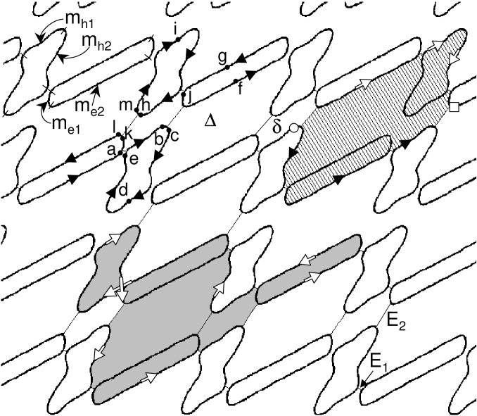
The room temperature FS of (ET)₈Hg₄Cl₁₂(C₆H₅Cl)₂ results from the hybridization of two pairs of hidden quasi-1D sheets 11 , parallel to the (a*, b* + c*) and (a*, c*) planes 12 ; 13 . The resultant FS, obtained after raising of degeneracy is built up with one hole and one elongated electron tube (see Figure 1). Although the cross section area of both electron and hole tubes amounts to 13 percent of the FBZ area 13 , the resulting orbits do not share the same topology and are separated from each other by two unequal gaps labeled E₁ and E₂ in Figure 1. Provided these gaps are not too large, MB between electron and hole orbits can occur in magnetic field, leading to a two-dimensional network of coupled orbits. This may give rise, besides quantum oscillations linked to the electron and hole closed orbits, to additional oscillation frequencies that can be accounted for either by the semiclassical model of Falicov and Stachowiak 4 or by QI. Regarding the FS topology at low temperature, it is worth to notice that a metallic groundstate is stabilized in (ET)₈Hg₄Cl₁₂(C₆H₅Cl)₂. Indeed, the conductivity exhibits a metallic behavior down to the lowest temperatures with a residual resistivity ratio equal to 1̃00 and without any sign of (even imperfect) nesting of neither electron nor hole tubes 12 .

Previous magnetoresistance experiments performed up to 15 teslas on (ET)₈Hg₄Cl₁₂(C₆H₅Cl)₂ crystals with the current injected within the conducting bc-plane (in-plane configuration) 14 exhibit one Shubnikov-de Haas (SdH) oscillation series, referred to as the a series hereafter, with a frequency F_a = 250 T corresponding to a cross section of $\approx$ 11 % of the FBZ area 14 . Nevertheless, when the current is injected in the direction a*, normal to the conducting plane (interlayer configuration), a complex oscillatory behavior is observed, in particular at high magnetic field 15 . Namely, in addition to a frequency F_b = 2200 T, corresponding to $\approx$ 100 % of the FBZ area, other frequencies which are linear combinations of the frequencies F_a = 240 T and F_δ = 150 T (7 % of the FBZ area), respectively have been observed.

The aim of this paper is to show that the oscillatory behavior of the interlayer magnetoresistance of the (ET)₈Hg₄Cl₁₂(C₆H₅Cl)₂ organic conductor results from several contributions, including MB-induced QI effects. This will be achieved through the analysis of the temperature and field magnitude and orientation dependencies of the oscillation spectrum.

II Experimental

The studied crystal was a platelet with approximate dimensions (1$\times$1$\times$0.1) mm³, the largest faces being parallel to the conducting bc-plane. Electrical contacts were made to the crystal using annealed gold wires of $20$ mm in diameter glued with graphite paste. Alternating current ($400$ mA, $50$ kHz) was injected parallel to the a* direction (interlayer configuration). A lock-in amplifier with a time constant of 100 ms was used to detect the signal across the potential leads. If the measurements, performed during the decay of the pulsed fields of the LNCMP ($36$ T, $1.2$ sec) were noiseless, this should allow to derive reliable oscillatory data down to e. g. $11$ T and $1$ T for a frequency of $2200$ T and $150$ T, respectively (see Ref. 16 ).

Data analysis is based on Fourier transforms (FT) calculated with an elevated cosine window in a given field range from B_min to B_max. In the following, the amplitude of a given oscillation series at the mean field value B = 2 / (1/B_min + 1/B_max) is determined by the ratio of the amplitude of the FT to (1/B_min - 1/B_max). The orientation of the magnetic field is defined by the angle $\theta$ between the field direction and the normal to the conducting bc-plane. The sign of $\theta$ is arbitrary.

III Results and discussion

III.1 Oscillatory spectrum

Figure 2: Oscillatory part of the magnetoconductance at $\sim$ $1.7$ K for different orientations of the magnetic field. $\sigma_{bg}$ is the field-dependent background part of the conductivity. $\theta$ is the angle between the magnetic field direction and the normal to the conducting plane.

Figure 3: Fourier transforms deduced from data in Figure 2. The magnetic field window is 10 - 30 T and 20 - 35.2 T for Fig. 3a and Fig. 3b, respectively.

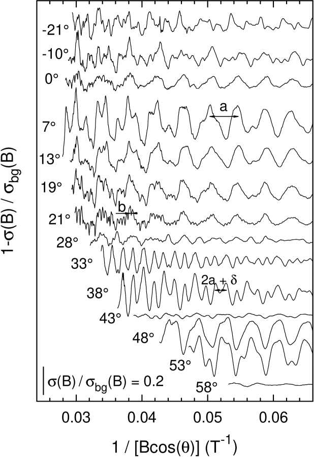
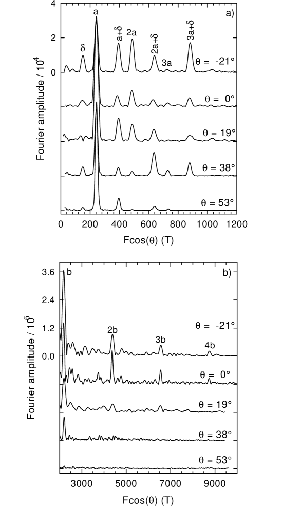
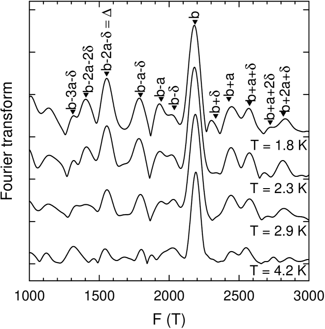
Fig. 2 displays the oscillatory magnetoconductance for different orientations of the magnetic field at a temperature of $\sim$ $1.7$ K. FT deduced from data in Fig. 2 are displayed in Fig. 3. A complex oscillatory behavior is observed since up to 6 fundamental frequencies - without counting some harmonics - are displayed in Fig. 3. Moreover, these 6 frequencies follow the orbital behavior expected for a two-dimensional FS in the explored angle range from -21^∘ to +72^∘, as demonstrated in Fig. 3 for some angles. In the field range between 10 and 30 teslas (see Figure 3a), the observed frequencies can be regarded as linear combinations of F_a and F_δ with F_a = (241.5 $\pm$ 2.0) T and F_δ = (149 $\pm$ 2) T. In addition, an oscillation series with a frequency F_b = (2185 $\pm$ 15) T and up to 3 harmonics are observed in the higher field range between 20 and 35.2 T (see Figure 3b). These three frequencies correspond to cross section area of 11.0 $\pm$ 0.1, 6.8 $\pm$ 0.1 and 100 $\pm$ 1 percent of the FBZ area, respectively. According to band structure calculations, the cross section area of the electron and the hole orbits corresponds to approximately 13 % of the FBZ area 13 . Keeping in mind that a discrepancy of few percents between experimental data and band structure calculations is an usual feature, it can be assumed that the calculated FS is in qualitative agreement with the experimental data. Hence F_a is associated to the closed electron and hole orbits (referred to as the a orbits in the following) and F_δ to the $\delta$ orbit. F_b, which corresponds to the whole FBZ area, accounts for an orbit that involves 2a + $\Delta$ + $\delta$. Owing to the experimental values of the frequencies F_a and F_δ, the cross section of the $\Delta$ orbit amounts to 71 % of the FBZ area. Finally, it is important to notice that more than ten frequency combinations involving F_b are also observed in FT performed in the high field range (see Fig. 4). In particular, the frequency linked to b-2a-$\delta$, which corresponds to the $\Delta$ orbit is clearly evidenced in the figure. In order to assign the above reported frequencies to k-space SdH orbits or QI paths, it is important to keep in mind that, following Falicov and Stachowiak 4 and Shoenberg 5 , areas enclosed by electron and hole parts of a MB orbit bears opposite sign. One of the possible consequence is that very large SdH orbits and QI paths including both electron and hole parts may account for a given (even rather low) frequency, although with a reduced damping factor and a large effective mass, as discussed in the next section. For example, F_δ can be attributed, among others, to both the semiclassical MB closed orbit (a b c d e b f g h m i h l a) and the QI path (a k l)-(a b c d e b f g h l) (see Fig. 1). It is worth to note that magnetic interaction MI can also induce frequency combinations in dHvA oscillations spectrum when the FS is composed of several orbits. However, recent measurements 17 have revealed that, as it is usually the case for most organic conductors, the value of the magnetization of the isostructural compound (ET)₈Hg₄Cl₁₂(C₆H₅Cl)₂ remains rather weak even at high magnetic field. This latter result makes unlikely a significant contribution of MI to the oscillation spectrum. In the following, we will examine the possible contribution of QI and conventional SdH effect to the observed oscillatory behavior through the temperature and magnetic field dependencies of the oscillation amplitude. Unfortunately, the oscillation series resulting from frequency combinations involving the F_b frequency (see Fig. 4) will not be considered due to too small amplitude and (or) too steep field and temperature dependencies.

Figure 4: Fourier transforms deduced from data at different temperatures for $\theta$ = 0^∘ in the magnetic field range 18 - 35.7 T. Frequency combinations involving a, b and $\delta$ orbits are indicated in the figure. Full triangles are marks calculated with F_a = 241.5 T, F_δ = 149 T and F_b = 2185 T. Note that the oscillation series b-2a-$\delta$ corresponds to the $\Delta$ orbit.

III.2 Calculation of effective masses and damping factors

According to the conventional Lifshitz-Kosevich (LK) model, the field and temperature dependence of the oscillatory part of the conductivity can be accounted for by:

$$1-\frac{\sigma(B)}{\sigma_{{bg}}(B)}=\sum_{{i}}A_{i}\cos\left[2\pi\left(\frac{F_{i}}{B}-\gamma_{i}\right)\right]$$ (1)

where $\sigma_{bg}$(B) is the field-dependent monotonous part of the conductivity. i stands for the indices of the oscillation series and $\gamma_{i}$ is the Onsager’s phase factor. Harmonics contribution can be included in the equation. Neglecting the spin splitting damping term, the oscillation amplitude A_i is given by:

$$A_{{i}}\propto R_{{T}}(i)R_{{D}}(i)R_{{MB}}(i)$$ (2)

where R_T and R_D are the temperature and Dingle damping terms, respectively. R_MB, which will be considered latter on, is the damping term which accounts for the contribution of MB. As usual, the Dingle damping term is expressed as:

$$R_{{D}}(i)=exp\left[-\frac{u_{{0}}T_{{D}}(i)m_{{c}}(i)}{B}\right]$$ (3)

where (u₀ = 14.694 T/K); T_D(i) and m_c(i) are the Dingle temperature and the effective cyclotron mass, respectively. R_T(i) is given by:

$$R_{{T}}(i)\propto\frac{Tm_{{c}}(i)/B^{n}}{\sinh\left[-u_{{0}}Tm_{{c}}(i)/B\right]}$$ (4)

In the two- and three-dimensional case, n is equal to 1 and 1/2, respectively 5 .

Following Falicov and Stachowiak 4 , the effective mass linked to electron and hole orbits can be expressed as m*_e = 2(m_e1 + m_e2) and m*_h = 2(m_h1 + m_h2), respectively. The weight factors m_e1, m_e2, m_h1 and m_h2, which can be regarded as absolute values of partial cyclotron mass parameters, are defined in Fig. 1. Since the oscillation series with frequency F_a results from the contribution of the electron and hole orbits, the resultant effective cyclotron mass has been assumed equal to m*_a = (m*_e + m*_h) / 2, i.e. m*_a = m_e1 + m_e2 + m_h1 + m_h2. Same type of calculation has been performed for the other SdH orbits as reported in Table 1.

Table 1: Experimental data and calculated parameters relevant to the observed oscillation series. F($\theta$ = 0^∘) is the oscillation frequency deduced from experimental data for the magnetic field applied perpendicular to the conducting plane. m* and m_c are the calculated effective mass and the experimental effective cyclotron mass deduced from the conventional LK model (in the temperature range below 8 K for b and $\delta$ oscillations), respectively relevant to the considered oscillation series. The field-dependent part of the damping factors K_SdH and K_QI are defined in Eq. (5) and (6), respectively. Only the SdH orbits and QI paths yielding the highest damping factors are considered in the table.

	Experimental data			Calculations
				SdH oscillations		Quantum interference oscillations
orbit	F($\theta=0^{\circ}$)	mc	mc/mc(a)	m*/m*(a)	KSdH	m*/m*(a)	KQI
$\delta$	149 $\pm$ 2	0.50 $\pm$ 0.15	0.43 $\pm$ 0.18	4	q${}_{1}^{6}$q${}_{2}^{4}$p${}_{1}^{2}$p${}_{2}^{2}$	2	$q_{1}^{4}q_{2}^{4}p_{1}^{2}p_{2}^{2}$
a	241.5 $\pm$ 2	1.17 $\pm$ 0.13	1	1	$q_{1}^{2}q_{2}^{2}$	not relevant	not relevant
a+$\delta$	391 $\pm$ 4	1.02 $\pm$ 0.08	0.87 $\pm$ 0.17	3	$q_{1}^{4}q_{2}^{4}p_{1}^{2}p_{2}^{2}$	1	$q_{1}^{2}q_{2}^{2}p_{1}^{2}p_{2}^{2}$
2a+$\delta$	633 $\pm$ 4	1.95 $\pm$ 0.10	1.67 $\pm$ 0.27	2	$q_{1}^{2}q_{2}^{2}p_{1}^{2}p_{2}^{2}$	2$\left|m_{e2}-m_{h2}\right|/m*(a)$	$q_{1}^{2}q_{2}^{2}p_{1}^{2}p_{2}^{2}$ or $q_{1}^{4}q_{2}^{2}p_{1}^{2}p_{2}^{2}$
3a+$\delta$	875 $\pm$ 15	0.73 $\pm$ 0.15	0.62 $\pm$ 0.20	3	$q_{1}^{4}q_{2}^{4}p_{1}^{2}p_{2}^{2}$	1	$q_{1}^{4}q_{2}^{4}p_{1}^{2}p_{2}^{2}$
b	2185 $\pm$ 15	0.5 $\pm$ 0.1	0.43 $\pm$ 0.13	4	$q_{1}^{6}q_{2}^{2}p_{1}^{2}p_{2}^{6}$	0	$q_{2}^{4}p_{1}^{4}p_{2}^{2}$ or $q_{1}^{4}p_{1}^{2}p_{2}^{4}$

In the framework of the QI model 2 ; 3 , the effective mass is given by the energy derivative of the phase difference ($\varphi_{i}$ - $\varphi_{j}$) between the two different routes i and j of a two-arm interferometer. Within this model, $\partial(\varphi_{i}-\varphi_{j})/\partial\epsilon=heB~{}\partial S_{k}/\partial\epsilon$, where S_k is the reciprocal space area bounded between the two arms. Since $\partial(\varphi_{i}-\varphi_{j})/\partial\epsilon$ is proportional to the difference between the effective mass of the two arms of the interferometer, the associated effective mass is given by m* = $\mid$ m*_i - m*_j $\mid$ where m*_i and m*_j are the partial effective masses of the routes i and j. The calculated values for the QI orbits are given in Table 1. It should be kept in mind that a given oscillation series can be accounted for by several types of QI paths or SdH orbits with different damping factors. Data in Table 1 is restricted to orbits yielding the highest damping factors i. e. with the lowest number of MB junctions and the lowest effective mass.

For a given oscillation series, noticeable differences between effective masses linked to either SdH or QI can be observed. E. g. m*_2a+δ is equal to 2 m*_a in the case of SdH while m*_2a+δ is equal to 2$\mid m_{e2}-m_{h2}\mid$ in the case of QI which is certainly much lower than m*_a.

We discuss now the damping factor R_MB entering Eq. (2). According to Falicov and Stachowiak 4 , the damping factor for a SdH orbit can be written as:

$$R_{MB}^{SdH}(i)=\prod_{g=1,2}p_{g}^{n_{pg}}q_{g}^{n_{qg}}\exp\left[i\left(n_{pg}\varphi_{p}+n_{qg}\varphi_{q}\right)\right]$$ (5)

The indices g stand for the two different gaps between electron and hole orbits (see Fig. 1). $\varphi_{p}$ and $\varphi_{q}$ are phase factors $(\varphi_{p}+\varphi_{q}=\pm\pi/2)$. The integers n_pg and n_qg are respectively equal to the number of MB and Bragg reflections encountered along the path of the quasiparticle. The MB and Bragg reflection probabilities are given by $p_{g}^{2}=exp(-B_{g}/B)$ and $\mid q_{g}\mid^{2}=1-p_{g}^{2}$ , respectively where B_g is the gap-dependent MB field. In the following, the field-dependent part of $R_{MB}^{SdH}(i)$ is expressed as K${}_{SdH}(i)=\prod_{g=1,2}p_{g}^{n_{pg}}q_{g}^{n_{qg}}$.

In the case of a two-arm interferometer, the damping term for QI is given, according to Harrison et al. 7 ; 18 by:

$${}R_{MB}^{QI}(i)\propto\prod_{k,g=1,2}p_{kg}^{n_{pg}}q_{kg}^{n_{qg}}\exp\left(-\frac{\pi}{\omega_{i}\tau_{t}}\right)$$ (6)

In this expression, i and g indices have the same meaning as in Eq. (5) while k indices stands for each of the two arms of the interferometer. n_pg and n_qg are the number of MB and Bragg reflections, respectively encountered by each of the arms of the interferometer. As stated in 18 , the relevant effective mass m_i entering $\omega_{i}=\hbar eB/m_{i}$ is the sum of the partial effective masses of the two branches of the interferometer. In addition, as pointed out by Stark and Friedberg 3 and contrary to the scattering time involved in the Dingle damping factor, which is usually assumed temperature-independent, the quantum state lifetime $\tau_{t}$ includes the temperature-dependent electron-phonon interaction. Assuming, that 1/$\tau_{t}$ is proportional to the zero field resistivity $\rho_{0}$(T) yields:

$$R_{MB}^{QI}(i)\propto K_{QI}(i)\exp\left(-\alpha(i)\rho_{0}\right)$$ (7)

where $\alpha$(i) and $\rho_{0}$ are field- and temperature-dependent, respectively.

As pointed out above and contrary to the case of e. g. $\kappa$-(ET)₂Cu(NCS)₂, several QI paths or SdH orbits with different topologies may contribute to a given oscillation series, even restricting ourselves to the orbits or paths with the highest damping factor. As an example, the a+$\delta$ series can be accounted for by the QI paths with the arms (a k l) - (a b f g h l) and (e b c) - (e k m i j c) (see Fig. 1). Nevertheless, both of them include the same four MB and four Bragg reflections involving the small and the large gap between electron and hole orbit. This leads to the field-dependent part of the damping factor K${}_{QI}(a+\delta)=q_{1}^{2}q_{2}^{2}p_{1}^{2}p_{2}^{2}$ (see Eq. (6) and (7)). In addition to SdH orbits which may present either hole (c d e k m i j c orbit) or electron (a b f g h l a orbit) character, the 2a+$\delta$ series can be accounted for by the two interferometers with the arms (a k m i j) - (a b f g j) and (b f g h m) - (b c d e k m). However, contrary to the case of the a+$\delta$ series, these two QI orbits yield different damping factors, namely $q_{1}^{4}q_{2}^{2}p_{1}^{2}p_{2}^{2}$ and $q_{1}^{2}q_{2}^{4}p_{1}^{2}p_{2}^{2}$, respectively. Regarding the b oscillation series, it can be accounted for by semiclassical MB orbits, such as the one marked with shaded area in Fig. 1, with large effective mass and reduced MB damping factors (see Table 1). A lot of QI paths can also account for F_b, even without taking into account the interferometers which involve QI paths with strongly different arms length and bear reduced MB damping factors (12 MB junctions) and large effective mass (m* = 2m*(a)). Among those with a zero effective mass, some interferometers also involve a large number of MB junctions. Since they are the most probable, only those which involve 10 MB junctions (see the hatched area in Fig. 1) are considered in Table 1.

III.3 Data analysis

Figure 5: Oscillatory part of the magnetoconductance at different temperatures in the field range 21.7 to 36 T. The angle between the magnetic field direction and the normal to the conducting plane is $\theta$ = -13^∘.

Figure 6: Temperature dependence of the oscillation amplitude of some of the series observed in Fig. 5. The angle between the magnetic field direction and the normal to the conducting plane is $\theta$ = -13^∘. The mean field value is 29.57 T, 28.29 T, 29.57 T and 27.66 T, respectively for the a, a+$\delta$, 2a+$\delta$ and 3a+$\delta$ series. Solid lines are best fits to Eq. (4).

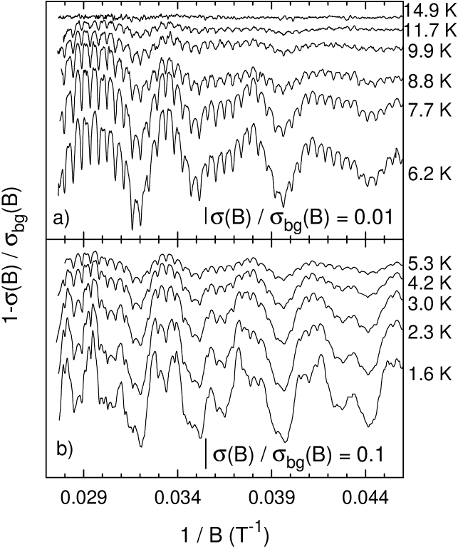
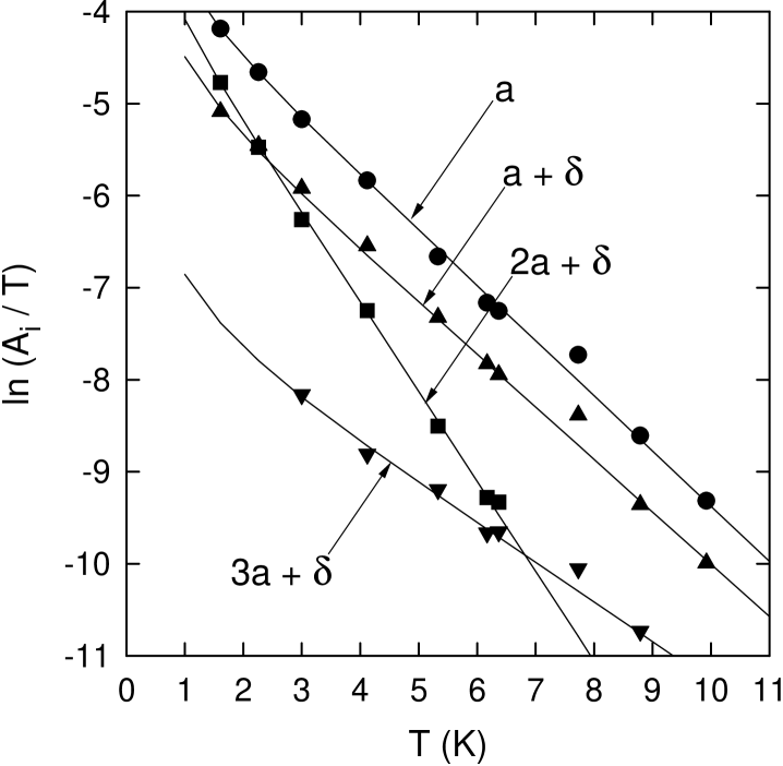
The oscillatory part of the magnetoconductance is displayed in the field range 22 to 36 T for $\theta$ = -13^∘ in Fig. 5. The temperature dependence of the amplitude of the oscillations for the a, a+$\delta$, 2a+$\delta$ and 3a+$\delta$ series observed in the oscillatory spectrum is displayed in Fig. 6 in the temperature range up to 10 K. A good agreement with the conventional LK model is observed as it is the case for the $\delta$ and b oscillations below $\sim$ 8K (see Fig. 7). However, Fig. 7 displays strong downward deviations from above $\sim$ 8 K for these latter series. These deviations from LK model are discussed later on. The cyclotron effective masses have been determined for different directions and mean values of the magnetic field. In the main, slight variations of the measured effective cyclotron mass parameter can be observed at high magnetic field, likely due to the strongly two-dimensional character of the FS 19 . Stronger downward deviations are nevertheless observed in some cases e. g. for m_c(a) at $\theta$ = 33^∘ and m_c(a+$\delta$) at $\theta$ = 22^∘. The values deduced from experimental data are given in Table 1, assuming that reliable values of the effective cyclotron mass are obtained at low magnetic field.

In the framework of the Fermi liquid theory, effective cyclotron masses are renormalised by electron-phonon interactions and electron correlation, accounted for by multiplicative factors (1 + $\lambda_{e-ph}$) and (1 + $\lambda_{e-e}$), respectively where $\lambda_{e-ph}$ and $\lambda_{e-e}$ are the strength of the interactions. Assuming this model holds in the present case, allows us to compare experimental values of m_c(i) / m_c(a) to calculated values of m*_i / m*_a.

Figure 7: Temperature dependence of the amplitude of the b (full circles) and $\delta$ (full squares) oscillations. The mean field value is 22.66 T and 29.57 T, respectively for the $\delta$ and b series. The angle between the magnetic field direction and the normal to the conducting plane is $\theta$ = -13^∘. Dashed lines are best fits to the LK model (see Eq. (4)) as done in Fig. 6. Full lines are best fits to the LK model, assuming a zero effective cyclotron mass and taking into account the temperature dependence of the quantum state lifetime according to Eq. (7). The temperature dependence of the zero field resistance (empty circles) is also displayed. Dotted line is a guide for the eye and accounts for a T^2.46 dependence (see text).

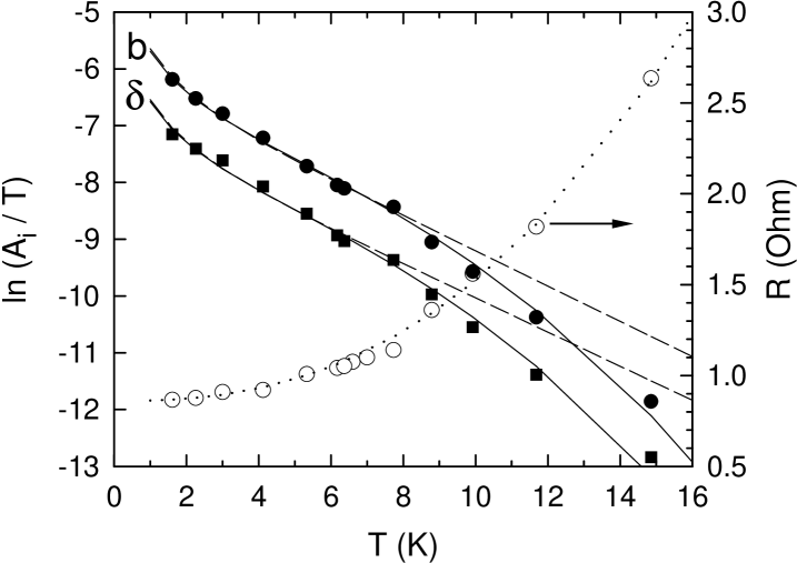
Effective cyclotron mass m_c(a+$\delta$) is close to m_c(a) (see Table 1) which is in agreement with QI phenomenon. Similarly, m_c(2a+$\delta$) value is in between m_c(a) and 2m_c(a) which suggests a significant contribution of conventional SdH. Oppositely, m_c($\delta$) and m_c(3a+$\delta$) are lower than m_c(a) which invalidates both the conventional SdH and the QI models. It must be pointed out that, the a+$\delta$ series is not observed in dHvA experiments performed at low magnetic field 15 , although these dHvA data present a better signal-to-noise ratio than the present conductivity data. This result suggests that QI do contribute to the oscillatory behavior. Otherwise, the 2a+$\delta$ frequency combination, which mainly results from SdH, is still visible in the dHvA experiment. Nevertheless, the frequencies linked to the $\delta$ and to the 3a+$\delta$ orbits which are not accounted for by neither conventional SdH nor QI are also not detected in the dHvA data. Owing to the large cross section of the b orbits, m_c(b) deduced from the low temperature part of the data is low when compared to m_c(a) since m_c(b) / m_c(a) $\sim$ 0.4 (see dashed lines in Fig. 7). This rules out the conventional SdH model and suggests that the b oscillation series may result from QI. Nevertheless, only the interferometers with a zero effective mass should significantly contribute to the oscillatory behavior. Such a discrepancy has already been observed in the case of the 3D LaB₆ compound which also exhibits a QI orbit with an extremal cross section equal to the FBZ area and for which a zero effective mass is predicted 18 . This discrepancy can be accounted for by Eq. (7) which assumes that the relevant lifetime arising in Eq. (6) is proportional to the interlayer conductivity in zero-field. This is demonstrated in Fig. 7 where solid lines are best fits to Eq. (2) assuming a zero effective cyclotron mass (i. e. R_T(b) defined in Eq. (4) is temperature-independent) and a temperature dependence of R${}_{MB}^{QI}$ given by Eq. (7). Even better agreement between data and Eq. (7) is obtained assuming 1/$\tau_{t}$ is proportional to T², which constitutes a signature of the Fermi liquid behavior. It can be noticed in Fig. 7 that Eq. (7) also holds for the $\delta$ oscillation series although there is no theoretical justification for this behavior in the framework of the SdH and QI models since much higher values of m_c($\delta$) are predicted in both cases (see Table 1).

Figure 8: Dingle plots of the oscillation series observed in the data at 1.6 K and $\theta$ = -13^∘ (see Fig. 5). Solid and dashed lines are best fits to the data taking and without taking into account contribution of magnetic breakdown damping factor, respectively (see text). The values of the effective cyclotron mass parameter m_c are given in Table 1.

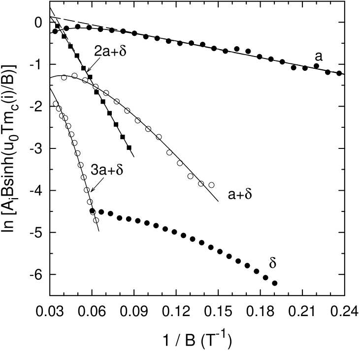
Additional information can be derived from the field dependence of the oscillation amplitude. Fig. 8 displays conventional Dingle plots of the various oscillation series at 1.6 K (see Fig. 5). Data at $\theta$ = -13^∘ have been chosen since no significant field dependence of the various effective cyclotron masses has been observed for this field direction. The b series has not been considered since reliable data can be derived for the b oscillations in a very narrow field range only, likely due to their weak amplitude. The two-dimensional case (n = 1 in Eq. (4)) is considered. Dashed lines in Fig. 8 are best fits of Eq. (2) to the data without taking into account any contribution of MB damping factor. Downward deviations from linearity are observed at high magnetic field 20 . Solid lines in the figure are best fits to the data including MB damping factor (see Table 1) relevant to either SdH (a and 2a+$\delta$ series) or QI (a+$\delta$ series). It is worth to note that the same damping factor holds for SdH and QI in the case of the 3a+$\delta$ oscillation series. Generally speaking, a very large uncertainty in the derived values of MB fields is obtained. Assuming same MB fields for the two gaps reduces the uncertainty and yields B₁ = B₂ = (55 $\pm$ 20) T for the a series. This value might also account for the data relevant to the 2a+$\delta$ series for which MB fields between 30 T and 160 T are obtained. Nevertheless, a negative Dingle temperature is obtained assuming MB field in this range even though the Dingle temperature for the a oscillation series is T_D(a) = 0.4 K. In addition, Dingle plot for the a+$\delta$ series can only be accounted for by lower MB fields i. e. between 0.2 T and 19 T (above 19 T, negative T_D values are obtained). Hence, the data in Fig. 8 cannot be accounted for by a unique set of MB field values. This may suggest that, in addition to SdH and QI, other contribution should play a role in the oscillatory data.

IV Summary and conclusion

The oscillatory behavior of the interlayer magnetoconductance of the quasi-two dimensional organic metal (BEDT-TTF)₈Hg₄Cl₁₂(C₆H₅Cl)₂ can be described on the basis of linear combinations of three basic frequencies arising from the compensated closed hole and electron orbits and from the two orbits located in between. It can be remarked first that the various MB-induced SdH orbits and QI paths responsible for the observed oscillation spectrum are not independent but do constitute an interlinked network which has been considered in the framework of the coupled orbits model of Falicov and Stachowiak 4 . On the basis of the derived values of the effective cyclotron masses linked to the various oscillation series, it can be inferred that a strong contribution of conventional SdH accounts for the 2a+$\delta$ series while data for a+$\delta$ and b, are consistent with QI. Oppositely, the low values of m${}_{c}(\delta)$ and m${}_{c}(3a+\delta$) disagree with both SdH and QI. In addition, the field dependence of the oscillation amplitude of the various series cannot be consistently accounted for by a unique set of MB gaps E₁ and E₂. These features suggest that additional contribution, such as frequency mixing due to oscillation of the chemical potential 7 ; 9 or interplay of electronic states from the different bands crossing the Fermi level 10 strongly influence the oscillatory behavior. From the experimental point of view, further enlightenment could be given by dHvA experiments in high magnetic field. Indeed, contrary to conductivity, magnetization, as a thermodynamic parameter, is not sensitive to QI. In addition, the configuration of measurement (in-plane vs. interlayer) should also be considered since, up to now, no frequency combinations has been observed in conductivity data recorded in the in-plane configuration 14 .

$\dagger$ author for correspondence: audouard@insa-tlse.fr

References

- (1) A. B. Pippard, Proc. Roy. Soc. (London) A270 1 (1962)
- (2) R. W. Stark and C. B. Friedberg, Phys. Rev. Lett. 26 556 (1971)
- (3) R. W. Stark and C. B. Friedberg, J. of Low Temp. Phys. 14 111 (1974)
- (4) L. M. Falicov and H. Stachowiak, Phys. Rev. 147 505 (1966)
- (5) D. Shoenberg, Magnetic Oscillations in Metals (Cambridge University Press, Cambridge, 1984)
- (6) F. A. Meyer, E. Steep, W. Biberacher, P. Christ, A. Lerf, A. G. M. Jansen, W. Joss, P. Wyder and K. Andres, Europhys. Lett. 32 681 (1995)
- (7) N. Harrison, J. Caulfield, J. Singleton, P. H. P. Reinders, F. Herlach, W. Hayes, M. Kurmoo and P. Day, J. Phys. Condens. Matter 8 5415 (1996)
- (8) M.V. Kartsovnik, G. Yu. Logvenov, T. Ishiguro, W. Biberacher, H. Anzai, N.D. Kushch, Phys. Rev. Lett, 77 2530 (1996)
- (9) J. Y. Fortin and T. Ziman, Phys. Rev. Lett. 80 3117 (1998)
- (10) P. S. Sandhu, J. H. Kim and J. S. Brooks, Phys. Rev. B 56 11566 (1997). J. H. Kim, S. Y. Han and J. S. Brooks, Phys. Rev. B 60 3213 (1999). S. Y. Han, J. S. Brooks and J. H. Kim, Phys. Lett. B 85 1500 (2000)
- (11) M.-H. Whangbo, J. Ren, W. Liang, E. Canadell, J.P. Pouget, S. Ravy, J. Williams, M.A. Beno, Inorg. Chem. 31, 4169 (1992)
- (12) R. N. Lyubovskaia, O. A. Dyachenko, V. V. Gritsenko, Sh. G. Mkoyan, L. O. Atovmyan, R. B. Lyubovskii, V. N. Laukhin, A. V. Zvarykina, and A. G. Khomenko, Synth. Metals 41 1907 (1991)
- (13) L. F. Vieros and E. Canadell, J. Phys. I France 4 939 (1994)
- (14) R. B. Lyubovskii, S. I. Pesotskii, A. Gilevskii and R. N. Lyubovskaia, JETP 80 946 (1995) [Zh. ksp. Teor. Fiz. 107 1698 (1994)] and J. Phys. I France 6 1809 (1996)
- (15) R. B. Lyubovskii, S. I. Pesotskii, C. Proust, V. I. Nizhankovskii, A. Audouard, L. Brossard and R. N. Lyubovskaia, Synth. Meth. 113 227 (2000)
- (16) C. Proust, A. Audouard, A. Kovalev, D. Vignolles, M. Kartsovnik, L. Brossard and N. Kushch, Phys. Rev. B 62 2388 (2000)
- (17) D. Vignolles et al. unpublished
- (18) N. Harrison, R. G. Goodrich, J. J. Vuillemin, Z. Fisk and D. G. Rickel, Phys. Rev. Lett. 20 4498 (1998)
- (19) See e. g. D. Vagner, T. Maniv and E. Ehrenfreund, Phys. Rev. Lett. 51 1700 (1983) and N. Harrison, R. Bogaerts, P. H. P. Reinders, J. Singleton, S. S. Blundell and F. Herlach, Phys. Rev. B 54 9977 (1996)
- (20) As already observed 21 , even stronger downward curvatures and lower slopes of the Dingle plots are obtained in the three-dimensional case (n = 1/2 in Eq. (4)). This leads to lower MB fields and Dingle temperature e. g. 30 T and 0.2 K, respectively for the a oscillation series
- (21) C. Proust, A. Audouard, V. Laukhin, L. Brossard, M. Honold, M.-S. Nam, E. Haanappel, J. Singleton and N. Kushch, Eur. Phys. J. B 21 31 (2001)