Coexistence of spin-triplet superconductivity and ferromagnetism induced by the local Hund’s rule exchange

Abstract

We characterize the coexistence of itinerant ferromagnetism and spin-triplet superconductivity within a single mechanism involving local (Hund’s rule) exchange among $d$ electrons. The ratio of transition temperatures and the spin anisotropy of the superconducting gap is estimated for $\rm ZrZn_{2}$. The $A$ phase is stable in very low applied and molecular fields, whereas the $A1$ phases persists in higher fields. A small residual magnetic moment is present below the Stoner threshold in the superconducting phase.

The coexistence of weak itinerant ferromagnetism (WFM) and superconductivity (SC) has been recently discovered in $\rm UGe_{2}$ (Ref. 1), $\rm ZrZn_{2}$ (Ref. 2) and $\rm URhGe$ (Ref. 3). The superconducting phase was encountered in the ferromagnetic phase; both of these phases seem to disappear with increasing pressure. Therefore, the superconductivity must be influenced by the ferromagnetism, particularly since the ratio of the Curie temperature $(T_{c})$ relative to the superconducting transition temperature $(T_{s})$ can exceed an order of magnitude.

It is hard to imagine that the superconducting pairing in that situation involves a spin singlet, since the molecular field, e.g., in $\rm ZrZn_{2}$ due to the exchange interaction, which is of the order of   [4] $H_{m}$ = 150 T $(\mu_{B}H_{m}$ = 17 meV), exceeds by far the thermodynamic critical field $H_{c}\leq 1\,T$.

In this paper we consider both of these types of ordering within a single mechanism – the Hund’s rule exchange and we draw some universal conclusions from a relatively simple and testable model containing two microscopic parameters (apart from the density of states and its derivatives at the Fermi level). We follow some of the approximations of the original Bardeen, Cooper, and Schrieffer (BCS) theory, although we employ the linearized dispersion relation and spin-split structure of quasiparticle states to account for the Fermi-liquid structure of the weak-ferromagnetic such as $\rm ZrZn_{2}$.

The $\it{spin-triplet}$ pairing in weakly ferromagnetic systems has been considered before being mediated by the exchange of longitudinal spin fluctuations [5] or being triggered by the electron-phonon interaction.[6]   Quite recently [7, 8], the question of the coexistence of ferromagnetism with $\it{spin-singlet}$ superconductivity has been reexamined within the mean-field theory. All the foregoing work is based on one-band (Hubbard or extended Hubbard) model, so the superconductivity can arise either from exchange of a paramagnon for repulsive interactions [5], or as a result of local attractive interaction ($\it negative-U\;model$).[7] In our approach the pairing, induced by local Hund’s’ rule exchange, appears in the correlated and orbitally degenerate systems and together with the short-range Coulomb interaction is regarded as the source of itinerant magnetism in 3d and 4d metallic system.  [11]This interorbital interaction remains local if the degenerate bands are not strongly hybridized. This is exactly what happens for $\rm ZrZn_{2}$, where the main contribution to the high density of states $\rho(\epsilon_{F})$ at the Fermi energy from the two $d$ bands, which do not hybridize [4, 12] (see also the discussion below.)

We start from the effective model proposed by us recently [10] and extend it to consider explicitly both ferromagnetism and superconductivity. It is represented by the Hamiltonian

$${\cal H}=\sum_{\mbox{\boldmath$k$}\ell\sigma}(E_{\mbox{\boldmath$k$}\ell}-\mu)n_{\mbox{\boldmath$k$}\ell\sigma}+{\cal H}_{ex}+{\cal H}_{c}$$ (1)

The quasiparticle band energy $E_{\mbox{\boldmath$k$}\ell}\equiv E_{\mbox{\boldmath$k$}\ell}-\mu$ of quasimomentum $k$ is labelled by the orbital index $\ell=1$ and 2. The local interorbital and intraatomic Hund’s’ rule coupling can be represented in two equivalent ways as [9]

$${\cal H}_{ex}=-2J\sum_{i}(\mbox{\boldmath$S$}_{i1}\cdot\mbox{\boldmath$S$}_{i2}+\frac{3}{4}n_{1i}n_{2i})=-2J\sum_{im}A_{im}^{+}A_{im},$$ (2)

where $\mbox{\boldmath$S$}_{i\ell}$ and $n_{i\ell}$ are the spin and the particle-number operators for $\ell$-th orbital on site $i$, and $a_{im}^{+}$ are real-space spin-triplet creation operators on site $i$ $(A_{i1}^{+}=a_{i1\uparrow}^{+}a_{2i\uparrow}^{+}$, etc.). ${\cal H}_{c}$ represents the direct Coulomb interaction (the Hubbard term), as well as the interorbital Coulomb term

$${\cal H}_{c}=U\sum_{li}n_{li\uparrow}n_{li\downarrow}+U^{\prime}\sum_{l\neq l^{\prime},i}n_{li}n_{li}\;.$$ (3)

The last term does not influence the phases considered in the first order so it is dropped out. So, (1) represents, in our view, a correlated system [13], in which the local interactions determine the quantum instabilities.

We introduce the combined Hartree-Fock-BCS approximation and the four dimensional Nambu-type representation. This means that the interaction part is rewritten first (up to a constant) in the following manner

$${\cal H}_{ex}+{\cal H}_{c} = -2J\sum_{m}\left(<A_{im}>A_{im}^{\dagger}+<A_{im}^{\dagger}>A_{im}-|<A_{im}>|^{2}\right)$$ (5)

$$-I\left[\sum_{i}\overline{S^{z}}(S_{i1}^{z}+S_{i2}^{z})-\frac{1}{2}(\overline{S^{z}})^{2}\right],$$

where $\overline{S^{z}}\equiv<S_{i1}^{z}+S_{i2}^{z}>$ is the magnetic moment per atom, $<A_{im}>$ is one of the three possible components of the superconducting gap parameters, and $I=U+2J$ is the effective Stoner parameter. Subsequently, the Hamiltonian can be rewritten as a $4\times 4$ matrix with creation operators ${\bf f}_{\mbox{\boldmath$k$}}^{+}\equiv(f_{\mbox{\boldmath$k$}1\uparrow}^{\dagger}f_{\mbox{\boldmath$k$}1\downarrow}^{\dagger},f_{-\mbox{\boldmath$k$}2\uparrow},f_{-\mbox{\boldmath$k$}2\downarrow})$, so that

$${\cal H} = \sum_{\mbox{\boldmath$k$}}\mbox{\boldmath$f$}_{\mbox{\boldmath$k$}}^{\dagger}\mbox{\boldmath$A$}\mbox{\boldmath$f$}_{\mbox{\boldmath$k$}}+\sum_{\mbox{\boldmath$k$}\sigma}E_{\mbox{\boldmath$k$}2}+N\left[I(\overline{S^{z}})^{2}+\sum_{m}\frac{|<A_{im}>|^{2}}{2J}\right],$$ (6)

where $A$ is $4\times 4$ matrix of the form

$$\mbox{\boldmath$A$}=\left(\begin{array}[]{ccccccc}E_{\mbox{\boldmath$k$}1}-I\overline{S^{z}}&,&0&,&\Delta_{1}&,&\Delta_{0}\\ 0&,&E_{\mbox{\boldmath$k$}1}+I\overline{S^{z}}&,&\Delta_{0}&,&\Delta_{-1}\\ \Delta_{1}&,&\Delta_{0}&,&-E_{\mbox{\boldmath$k$}2}+I\overline{S^{z}}&,&0\\ \Delta_{0}&,&\Delta_{-1}&,&0&,&-E_{\mbox{\boldmath$k$}2}-I\overline{S^{z}}\end{array}\right).$$

This matrix can be diagonalized analytically. The interesting cases are only those with the spin dependend gaps (i) $\Delta_{\uparrow}>\Delta_{\downarrow}$ and $\Delta_{0}=0$ (which we call the anisotropic $A$ phase); and (ii) $\Delta_{\uparrow}\neq 0$ and $\Delta_{\downarrow}=\Delta_{0}=0$ (which is called the $A1$ phase). In case (i), the four eigenvalues are

$$\lambda_{\mbox{\boldmath$k$}\sigma 1,2}=\frac{1}{2}(E_{\mbox{\boldmath$k$}1}-E_{\mbox{\boldmath$k$}2})\mp\left[\frac{1}{4}(E_{\mbox{\boldmath$k$}1}+E_{\mbox{\boldmath$k$}2}-\sigma I\overline{S^{z}})^{2}+\Delta_{\sigma}^{2}\right]^{1/2}.$$ (8)

The sign $(\mp)$ corresponds to the labels (1,2) of $\lambda_{\mbox{\boldmath$k$}\sigma}$ and reflects hole and electron excitations, respectively. The spectrum is separated with respect to the spin orientation $\sigma=\pm 1$ of the Cooper pair. The spectrum is fully gapped if both $\Delta_{\uparrow}$ and $\Delta_{\downarrow}$ are nonzero. We obtain a combination of the spin splitting and superconducting gap (the gap at the Fermi energy $E_{F}=\mu$) is $2\left(\sqrt{(I\overline{S^{z}})^{2}+\Delta_{\uparrow}^{2}}+\sqrt{(I\overline{S^{z}})^{2}+\Delta_{\downarrow}^{2}}\right)\sim 2I\overline{S^{z}}$ when the spin is flipped and $\Delta_{\uparrow}$ or $\Delta_{\downarrow}$ within the spin subband. What is probably more important, in $A1$ state half of the spectrum remains gapless $\lambda_{\mbox{\boldmath$k$}\downarrow 1}=-E_{\mbox{\boldmath$k$}2}+I\overline{S^{z}}$, $\lambda_{k\downarrow 2}=E_{\mbox{\boldmath$k$}1}+I\overline{S^{z}}$. Thus, there should be a substantial linear specific-heat term present also in the superconducting $A1$ state and this dependence should be distinguished from the $T^{n}$ dependence $(n\geq 2)$ due to the gap zeros (the latter would require the interband hybridization and hence the dependence [14] $J\rightarrow J_{\mbox{\boldmath$k$}\mbox{\boldmath$k$}^{\prime}})$. The linear specific heat $\gamma$ comes from the spin minority electrons, and since for a weak itinerant magnet $I\overline{S^{z}}\ll E_{F}$, there will be drop in the relative value of $\gamma$ of the order $\rho_{\downarrow}/(\rho_{\uparrow}+\rho_{\downarrow})$, where $\rho_{\sigma}\equiv\rho_{\sigma}(E_{F})$ is the density of states in spin-$\sigma$ subband at the Fermi energy.

The results obtained so far are general in the sense they are independent of a particular electronic structure. In the following we assume that the bands are the same, i.e. $E_{\mbox{\boldmath$k$}1}=E_{\mbox{\boldmath$k$}2}\equiv E_{\mbox{\boldmath$k$}}$ so that $E_{\mbox{\boldmath$k$}}-\mu\simeq{\mbox{\boldmath$v$}}_{F}\mbox{\boldmath$k$}$, where $v_{F}$ is the Fermi velocity.

The Bogolyubov quasiparticle operators can also be easily calculated; then they are [15]

$$\left(\begin{array}[]{cc}\alpha_{\mbox{\boldmath$k$}\sigma}\\ \beta_{-\mbox{\boldmath$k$}\sigma}^{\dagger}\end{array}\right)=\frac{1}{\sqrt{2}}\left(\begin{array}[]{ccc}u_{\mbox{\boldmath$k$}}^{(\sigma)}&,&v_{\mbox{\boldmath$k$}}^{(\sigma)}\\ -v_{\mbox{\boldmath$k$}}^{(\sigma)}&,&u_{\mbox{\boldmath$k$}}^{(\sigma)}\end{array}\right)\left(\begin{array}[]{c}f_{\mbox{\boldmath$k$}1\sigma}+f_{-\mbox{\boldmath$k$}2\sigma}^{\dagger}\\ f_{\mbox{\boldmath$k$}1\sigma}-f_{-\mbox{\boldmath$k$}2\sigma}^{\dagger}\end{array}\right),$$ (15)

with the coherence factors

$$\left(\begin{array}[]{c}u_{\mbox{\boldmath$k$}}^{(\sigma)}\\ v_{\mbox{\boldmath$k$}}^{(\sigma)}\end{array}\right)=\frac{1}{\sqrt{2}}\left(\begin{array}[]{ll}1+\Delta_{\sigma}/\lambda_{\mbox{\boldmath$k$}\sigma}\\ 1-\Delta_{\sigma}/\lambda_{\mbox{\boldmath$k$}\sigma}\end{array}\right),$$ (20)

and the eigenvalue $\lambda_{\mbox{\boldmath$k$}\sigma}=\lambda_{\mbox{\boldmath$k$}\sigma 1}=-\lambda_{\mbox{\boldmath$k$}\sigma 2}\equiv[(v_{\sigma}k)^{2}+\Delta_{\sigma}^{2}]^{1/2}$. Note that the spin dependent Fermi velocity is caused by the circumstance that we have spin-split bands in the ferromagnetic phase. The Hamiltonian has the diagonal form ${\cal H}=\sum_{\mbox{\boldmath$k$}\sigma}\lambda_{k\sigma}(\alpha_{\mbox{\boldmath$k$}\sigma}^{+}\alpha_{\mbox{\boldmath$k$}\sigma}+\beta_{-\mbox{\boldmath$k$}\sigma}\beta_{-\mbox{\boldmath$k$}\sigma})+E_{0}$, which is the BCS form with spin-dependent quasiparticle and gap energies. The last factor contributes to important differences with the BCS theory. Namely, the gap parameter at temperature $T=0$ is determined from the equation

$$1=J\rho_{\sigma}\int_{-k_{m\sigma}}^{k_{m\sigma}}\frac{d^{3}(v_{\sigma}\mbox{\boldmath$k$})}{\sqrt{(v_{\sigma}k)^{2}+\Delta_{\sigma}^{2}}},$$ (21)

where $\rho_{\sigma}=12\epsilon_{F\sigma}^{2}/W$ $(\epsilon_{f\sigma}$ is the Fermi energy for quasiparticles with spin $\sigma$ and $W$ is the effective width of the band, related to the Fermi velocity via $W=(24\pi^{2}\hbar v_{F}^{2}/\Omega_{0})^{1/3}$, where $\Omega_{0}$ is the elementary-cell volume). The integration boundary $k_{m}$ is determined by the condition that the paired particles with spin $\sigma$ are present only within the spin-split region of the band, i.e., by the constraint $v_{\sigma}k_{m\sigma}=\sigma I\overline{S^{z}}$. In effect, we obtain an estimate

$$\Delta_{\sigma}=4I\overline{S^{z}}\exp\left(-\frac{1}{\rho_{\sigma}J}\right).$$ (22)

Analogously, we can estimate the critical temperature by selecting an equivalent but slightly different representation of the quasiparticle energies: $E_{\mbox{\boldmath$k$}}-\mu-\sigma I\overline{S^{z}}=\hbar v_{F}k-\sigma I\overline{S^{z}}$, where $v_{F}$ is the Fermi velocity in the paramagnetic phase. Then the condition for $T_{S}$ (for $\Delta=\Delta_{\uparrow})$ reduces to

$$1=I\int_{-k_{min}}^{k_{min}}\frac{\tanh\left(\frac{\hbar v_{F}k-2J\overline{S^{z}}}{2k_{B}T_{S}}\right)}{\hbar v_{F}k-J\overline{S^{z}}}.$$ (23)

In effect, we obtain the estimate

$$k_{B}T_{S}\simeq 2.26I\overline{S^{z}}\exp\left(-\frac{1}{J\rho}\right).$$ (24)

In both expressions for $\Delta_{\sigma}$ and for $T_{S}$, the exponent contains the exchange integral, whereas the preexponential factor is multiplied by the magnetic moment. This means that spin-triplet superconductivity disappears together with ferromagnetism. This result is more general as it relies on the well founded notion that Cooper per of spin orientation $\sigma$ exist within the corresponding spin subbands if only $\Delta_{0}=0$ (the B phase is not stable).

To make the estimates explicit we have to relate the results for a weak itinerant ferromagnet.  [16] It is easy to rederive those results in the present situation with $T_{c}\gg T_{S}$. Namely, the Curie temperature is given by the expression

$$T_{c}=\frac{\sqrt{6}}{\pi}\left[\left(\frac{\rho^{{}^{\prime}}}{\rho}\right)^{2}-\frac{\rho^{\prime\prime}}{\rho}\right]^{-1/2}[(I\rho-1)/I\rho]^{1/2},$$ (25)

with $\rho^{\prime}$ and $\rho^{\prime\prime}$ being, respectively, the first and the second derivative of the density of states $\rho(E)$ taken at $E_{F}$. Additionally, the magnetic moment at $T=0$ is given by $\overline{S^{z}}=(1/2)[(I\rho-1)/B]^{1/2}$, with

$$B=I^{\,3}\frac{\rho}{8}\left[\left(\frac{\rho^{\prime}}{\rho}\right)^{2}-\frac{\rho^{\prime\prime}}{\rho}\right].$$ (26)

Taking the parabolic density of states corresponding to the linearized dispersion relation, we can determine the ratio $T_{s}/T_{c}$ in an explicit manner

$$\frac{T_{S}}{T_{c}}\simeq 1.17\exp\left(-\frac{1}{J\rho}\right).$$ (27)

Similarly, the gap ratio is

$$\frac{\Delta_{\uparrow}}{\Delta_{\downarrow}}\simeq\exp\left((2I/3J)(\rho^{\prime}/\rho^{2})\overline{S^{z}}\right),$$ (28)

which in the limit $I\rho\approx 1$ gives the ratio exceeding three. The ratio will grow rapidly with $\overline{S^{z}}$ and the prediction $\ln(\Delta_{\uparrow}/\Delta_{\downarrow})\sim\overline{S_{z}}$ could be tested experimentally. The $A1$ superconducting state is reached fast with the increasing moment.

To interpret our findings in the coexistence regime we can say that the $A$ phase (with $\Delta_{\downarrow}\neq 0)$ cannot appear either near the quantum critical point – the Stoner threshold, at which $I\rho=1$, or in the ferromagnetically saturated state. In the former case, the relatively small field can polarize totally the system (since the magnetic susceptibility $\chi=\chi_{0}/(1-I\rho)$ is almost divergent). Under these circumstances, the bound state with $\Delta_{\downarrow}\neq 0$ cannot be formed, since the polarized surrounding will respond to the presence of the second electron strongly. On the other hand, if the magnetic moment in the ferromagnetic state is almost saturated, then the bound state with $\Delta_{\downarrow}$ cannot be formed as the system is rigid. Only in between those two limiting situations, but rather on the weak-ferromagnetic side, the coherent $A$ state can be realized. Otherwise, the $A1$ state will become stable.

To gain a quantitative insight into the nature of $A$ and $A1$ states and their coexistence with the spin polarized state, we have also performed the analysis in the paramagnetic state, i.e., for $\rho I<1$, but in the applied magnetic field $B\neq 0$. To amplify numerically the effects discussed,we have put $I=J$ and choose a constant density of states . The phase diagram as a function of magnetic field is displayed in Fig. 1. Note again that the phase $A$ disappears in the vicinity of the Stoner threshold marked by the vertical dashed line. On the contrary, the phase $A1$ continues towards the Stoner boundary. In Fig. 2, we provide the field dependence of the ground state energy away from the Stoner threshold for normal, $A$, and $A1$ phases. The $A1$ phase is the most stable in a high applied field and can coexist with a saturated ferromagnetism. The same happens for the superfluid $\rm{}^{3}He$. This means that the superconducting coherence length for $A1$ phase becomes unbound when the system reaches the saturated state.

The interesting feature of our results is that the presence of the superconductivity indices a magnetic moment even below the Stoner threshold. The magnitude of the moment below the Stoner threshold $(J/W=0.25$ in this case) is displayed in Fig. 3. Obviously, the effect is enhanced by the choice of the density of states selected and particularly by the assumption $I=J$ , but it is worth mentioning. It suggests that in the presence of the superconducting state makes the Stoner critical point a hidden one. This point will be elaborated further elsewhere.

In summary, we have considered the most natural model for the coexistence of ferromagnetism and spin-triplet superconductivity, both induced by a single mechanism – the local ferromagnetic exchange in the orbitally degenerate systems. While the anisotropic $A$-state seems to be stable in weakly polarized and paramagnetic systems at low fields, the $A1$ state may coexist even closer to the quantum critical point. The paired state induces a small magnetic moment even below the Stoner threshold. It should be interesting to extend these results to the hybridized systems [10], when $k$-dependent (p- or d-wave) spin-triplet superconductivity will appear.

This work was supported by the KBN Grant No. 2P03B 092 18, as well as by NSF Grant No. DMR 96-12130.

Figure Captions

Fig.1. Phase diagram specifying the stable superconducting states A and A1 (see main text). The dotted line specifies the onset of the magnetically saturated state. The vertical dot-dashed line marks the Stoner threshold.

Fig.2. Ground-state versus applied magnetic field B. At $B=0$ the equal-spin pairing state (A-phase) is stable, whereas in high field A1 phase (with the spins parallel) prevails. The system is below the Stoner threshold.

Fig.3. Magnetic moment per orbital (upper panel) and the superconducting gaps (lower panel) versus applied field (below the Stoner threshold). The inset shows the chemical potential vs. $B$. The horizontal arrow indicates a small residual magnetic moment in the $B\rightarrow 0$ limit below the Stoner threshold.

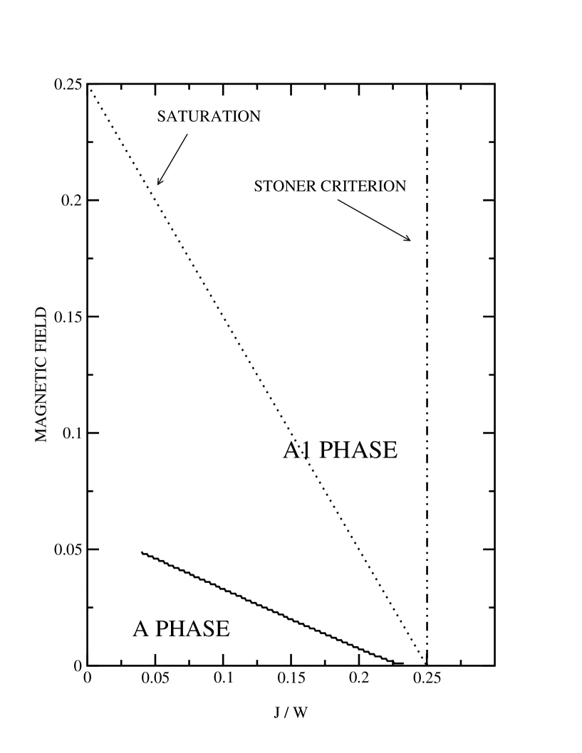
FIG. 1.:

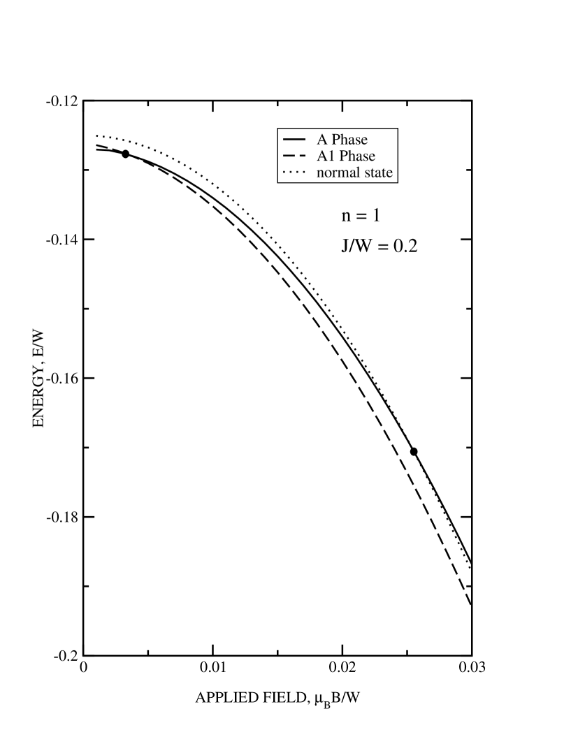
FIG. 2.:

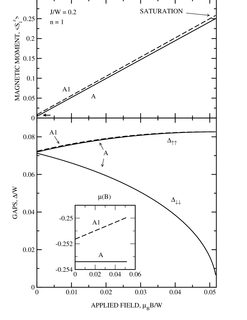
FIG. 3.:

REFERENCES

- [1] S. S. Saxena, et al., Nature 406, 587 (2000); A. Huxley, et al., Phys. Rev. B 63, 144519 (2001); N. Tateiwa et al., J. Phys. C 13, L17 (2001).
- [2] C. Pfeiderer, et al., Nature 412, 58 (2001).
- [3] D. Aoki et al., Nature 413, 613 (2001).
- [4] D. D. Koelling, D. L. Johnson, S. Kirkpatrick, and F. M. Mueller, Solid State Commun. 9, 2039 (1971).
- [5] D. Fay and J. Appel, Phys. Rev. B 22, 3173 (1980) and references therein.
- [6] C. P. Enz and B. T. Matthias, Science 201, 828 (1978); Z. Phys. B 33, 129 (1979).
- [7] N. I. Karchev, K. B. Blagoev, K. S. Bedell, and P. B. Littlewood, Phys. Rev. Lett. 86, 846 (2001), and references therein.
- [8] The recent work was preceded by: A. J. Larkin and Yu. N. Ovchinnikov, Zh. Eksp. Teor. Fiz. 47, 1136 (1964) [Sov. Phys. JETP 20, 762 (1965)]; P. Fulde and R. A. Ferrell, Phys. Rev. 135, A550 (1964).
- [9] A. Klejnberg and J. Spałek, J. Phys.: Cond. Matter 11, 6553 (1999). A similar model has been considered in the random phase approximation for the pairing by T. Takimoto, Phys. Rev. B 62, R14641 (2000).
- [10] J. Spałek, Phys. Rev. B 63, 104513 (2001).
- [11] For recent discussion of both factor see e.g. A.Klejnberg and J.Spalek, Phys. Rev. B 57, 12041 (1998); particularly pp.12049-50.
- [12] D. L. Johnson, Phys. Rev. B 9, 2273 (1974). Actually, they are somewhat hybridized with Zn electrons, which we ignore (cf. T. Jarlborg, A. J. Freeman, and D. D. Koelling, J. Magn. Mat. 23, 291 (1981)). See also: G. Santi, S. B. Dugdale, and T. Jarlborg, cond-mat/0107304.
- [13] The large value of = 47 mJ/mol K2 (Ref. 2) requires very large value of the many-body enhancement.
- [14] J. Spałek, unpublished.
- [15] We assume here that the Fermi velocities are the same in both bands (flat bands11), but they will depend on the spin so that we can represent the spin-split bands near in the form: .
- [16] E. P. Wohlfarth, J. Appl. Phys. 39, 1061 (1968). This theory provides an overall behavior of the properties. More refined theory invokes the spin fluctuations, (cf. T. Moriya, Spin Fluctuations in Itinerant-Electron Magnetism, Springer-Verlag, Berlin, 1985); this is not crucial for the estimates discussed here.
- [17] The details of density of states should not matter for qualitative features of the results, as we integrate now over the whole band states.