Potential Energy Landscape Equation of State

Abstract

Depth, number, and shape of the basins of the potential energy landscape are the key ingredients of the inherent structure thermodynamic formalism introduced by Stillinger and Weber [F. H. Stillinger and T. A. Weber, Phys. Rev. A 25, 978 (1982)]. Within this formalism, an equation of state based only on the volume dependence of these landscape properties is derived. Vibrational and configurational contributions to pressure are sorted out in a transparent way. Predictions are successfully compared with data from extensive molecular dynamics simulations of a simple model for the fragile liquid orthoterphenyl.

Recent years have seen a resurgence in studies devoted to modeling the thermodynamics of supercooled liquids thermo4 ; thermo3 ; angell ; thermo2 ; wales . Such studies aim to elucidate the physics of the liquid-glass transition, to develop a thermodynamic description of out of equilibrium systems and to provide keys for a deeper understanding of the dynamics of supercooled states debenedetti01 . Numerical studies, boosted by increased computational resources which now allow simulations to track the slowing down of the dynamics over more than 6 decades in time, are providing quantitative estimates for the free energy of simple model systems lennard_jones_pes ; heuer97 ; scala2000 ; sastry2001 . The availability of such data provides stringent tests of the theoretical predictions scala2000 ; sastry2001 ; ivannature and helps in the understanding of basic mechanisms associated with the behavior of thermodynamic and dynamic quantities close to the glass transition.

Among the thermodynamic formalisms amenable to numerical investigation, a central role is played by the Inherent Structure (IS) formalism introduced by Stillinger and Weber sw . Properties of the potential energy landscape (PEL), such as depth, number and shape of the basins of the potential energy surface are calculated and used in the evaluation of the liquid free energy scala2000 ; sastry2001 ; ivannature ; mossa02 In the IS formalism, the system free energy is expressed as a sum of an entropic contribution, accounting for the number of the available basins, and a vibrational contribution, expressing the free energy of the system when constrained in one of the basins sw .

Important progress has been made after the discovery that — for models of fragile liquids — the number $\Omega(e_{IS})$ of distinct basins of depth $e_{IS}$ in a system of $N$ atoms or molecules is well described by a Gaussian distribution sastry2001 ; heuer00

$$\Omega(e_{IS})=e^{\alpha N}\frac{e^{-(e_{IS}-E_{o})^{2}/2\sigma^{2}}}{(2\pi\sigma^{2})^{1/2}}.$$ (1)

Here the amplitude $e^{\alpha N}$ accounts for the total number of basins. Numerical studies of models for fragile liquids have also shown that the basin free energy can be written as the depth $e_{IS}$ plus a vibrational contribution which, in the harmonic approximation, has the well known form

$$F_{vib}(e_{IS},T)=k_{B}T\sum_{i=1}^{M}\ln(\beta\hbar\omega_{i}(e_{IS})),$$ (2)

where $\omega_{i}(e_{IS})$ is the $i$-th normal mode frequency ($i=1...M$) and $\beta=1/k_{B}T$. The $M$ normal mode frequencies define the shape of the basin. If relevant, anharmonic corrections can also be accounted for ivannature ; mossa02 . The quantity $\sum_{i=1}^{M}\ln(\omega_{i}(e_{IS})/\omega_{o})$ (where $\omega_{o}$ is the frequency unit) is found to depend linearly on the basin depth sastry2001 , i.e. can be written, in terms of two parameters $a$ and $b$, as

$$\sum_{i=1}^{M}\ln(\omega_{i}(e_{IS})/\omega_{o})=a+b\,e_{IS}.$$ (3)

Hence, the vibrational free energy can be written as

$$F_{vib}(e_{IS},T)=F_{vib}(E_{o},T)+k_{B}T\,b(e_{IS}-E_{o}).$$ (4)

Within the two assumptions of Eq. (1) — Gaussian distribution of basin depths — and Eq. (4) — linear dependence of the basin free energy on $e_{IS}$ — an exact evaluation of the partition function can be carried out. The corresponding Helmholtz free energy is given by sastry2001

$$F(T) = -TS_{conf}(T)+\langle e_{IS}(T)\rangle$$

$$+ F_{vib}(E_{o},T)+k_{B}T\,b(\langle e_{IS}(T)\rangle-E_{o}),$$

where

$$\langle e_{IS}(T)\rangle=(E_{o}-b\sigma^{2})-\beta\sigma^{2}=e_{\infty}-\beta\sigma^{2},$$ (6)

and

$$S_{conf}(T)/k_{B} = \alpha N-(\langle e_{IS}(T)\rangle-E_{o})^{2}/2\sigma^{2}$$ (7)

$$= S_{\infty}/k_{B}-b\,\beta\,\sigma^{2}-\beta^{2}\sigma^{2}/2.$$

In the above equations, $e_{\infty}$ and $S_{\infty}$ are defined as the value of $\langle e_{IS}\rangle$ and $S_{conf}$ at infinite $T$. Eqs. (Potential Energy Landscape Equation of State)-(7) show that, along constant volume $V$ paths, the behavior of the thermodynamic quantities is controlled by the values of the PEL properties, as given by $\alpha$, $\sigma$, $E_{0}$ (from Eq. (1)) and by $a$ and $b$ (from Eq. (3)).

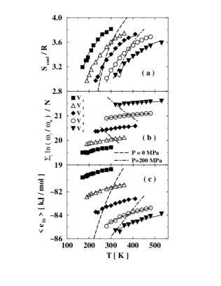
Figure 1: T dependence of (a) $S_{conf}$, (b) $\sum_{i}\ln(\omega_{i}/\omega_{o})/N$, and (c) $\langle e_{IS}\rangle$ (per molecule) at the five studied volumes $V_{k}$ (symbols). Data are from Ref. mossa02 . The full curves are simultaneous fits of the three sets of data according to Eqs. (7), (3), and (6). The dashed curves are the constant $P$ paths (at $P=0$ and $200$ MPa) calculated according to the IS-EOS as discussed in the text. The frequency unit is $\omega_{0}\equiv 1cm^{-1}$

In this Letter we study the volume dependence of Eq. (Potential Energy Landscape Equation of State) to provide an expression for the equation of state (EOS) based completely on landscape properties (PEL-EOS) debenedettieos . This study provides a significant insight into the understanding of the pressure $P$ and opens the way for detailed comparisons between experimental measurements (usually performed at constant $P$) and theoretical approaches based on the IS formalism. It may also help in developing an IS-based thermodynamic description of out-of-equilibrium (glass) states and a theoretical definition of the concepts of fictive $P$ and $T$aging .

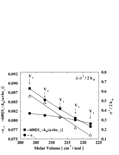
Figure 2: $V-$dependence of the three combinations of PEL parameters contributing to the linear (squares), constant (circles) and $T^{-1}$ (triangles) components of $P$, according to Eq. (11). The solid lines are the polynomial fit used to evaluate $P_{const}$, $P_{{}_{T}}$ and $P_{1/T}$. Tables of the coefficients of the polynomial fit will be reported in Ref. lanave02 . Here $e_{\infty}$ is expressed in $10^{6}J/mol$, $S_{\infty}-k_{B}(a+be_{\infty})$ in $10^{6}J/mol/K$, and $\sigma^{2}/2k_{B}$ in $10^{6}JK/mol$.

In thermodynamics, $P$ is defined as the (negative) $V$ derivative of the Helmholtz free energy. Hence $P$ if fully determined by the $V$ dependence of the landscape properties $\alpha$, $\sigma$, $E_{0}$, $a$ and $b$. Eq. (Potential Energy Landscape Equation of State) shows that $P$ can be split into three main contributions: a configurational one, $P_{conf}$ — related to the change in the number of available basins with $V$; an $e_{IS}$ one, $P_{e_{IS}}$ — related to the change in basin depth with $V$; and a vibrational one, $P_{vib}$ — related to the change in the shape of the explored basin with $V$. The $T$ dependence of each contribution can then be studied independently. The explicit expressions for these contributions are:

$$P_{conf}(T,V)=T\frac{\partial}{\partial V}S_{\infty}-\frac{\partial}{\partial V}(b\sigma^{2})-\frac{1}{T}\frac{\partial}{\partial V}(\sigma^{2}/2k_{B})$$ (8)

$$P_{e_{IS}}(T,V)=-\frac{\partial}{\partial V}e_{\infty}+\frac{1}{T}\frac{\partial}{\partial V}(\sigma^{2}/k_{B})$$ (9)

$$P_{vib}(T,V)=-k_{B}T\frac{\partial}{\partial V}(a+be_{\infty})+\frac{\partial}{\partial V}(b\sigma^{2}).$$ (10)

By grouping together all the contributions with the same $T$ dependence, $P$ can be expressed in term of $V$ derivatives of only three combinations of the five PEL parametersanomali

$$P(T,V)=P_{const}+TP_{{}_{{}_{T}}}+T^{-1}P_{{}_{{}_{1/T}}},$$ (11)

where $P_{const}=-\partial e_{\infty}/\partial V$, $P_{{}_{{}_{T}}}=\partial S_{\infty}/\partial V-k_{B}\frac{\partial}{\partial V}(a+be_{\infty})$ and $P_{{}_{{}_{1/T}}}=\frac{\partial}{\partial V}(\sigma^{2}/2k_{B})$.

The present formalism also provides an expression for the so-called inherent structure equation of state (IS-EOS), $P_{IS}(T_{IS},V)$ debenedettieos ; laviolette ; roberts ; sastry00 , i.e. the relation between the pressure and volume of the typical IS and the temperature $T_{IS}$ of the equilibrium ensemble from which configurations were extracted. Indeed, the constant $V$ steepest descent minimization procedure, which realizes the search for the closest local minimum starting from an equilibrium configuration, suppresses all the vibrational components (hence $P_{vib}=0$) but keeps $P_{conf}$ and $P_{e_{IS}}$ frozen at their “equilibrium” initial value. As a result $P_{IS}$, a purely mechanical quantity, can be expressed as

$$P_{IS}(T_{IS},V)=P_{conf}+P_{e_{is}}=$$

$$-\frac{\partial}{\partial V}E_{o}+T_{IS}\frac{\partial}{\partial V}S_{\infty}+\frac{1}{k_{B}T_{IS}}\frac{\partial}{\partial V}(\sigma^{2}/2).$$ (12)

Figure 3: Comparison between $P$ evaluated according to the $V$ derivative of PEL properties (lines) and $P$ evaluated in the MD simulation using the virial expression (symbols). Solid symbols are equilibrium values. For each $V_{k}$, the symbol $*$ indicates $P_{IS}$ for the coldest equilibrated state point. Open symbols are MD data calculated during a constant heating procedure starting from the IS configuration marked with $*$, as explained in the text. Lines are PEL-EOS for equilibrium (full lines, Eq. (11)) and for the heating procedure (dashed lines, Eq. (13)).

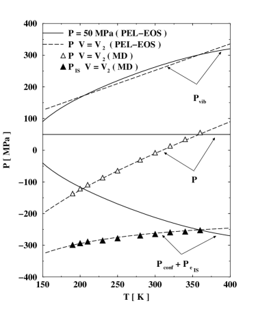
Figure 4: Total ($P$), vibrational ($P_{vib}$) and $e_{IS}$ plus configurational ($P_{e_{IS}}+P_{conf}$) contributions to $P$ along constant $V$ (dashed lines) and constant $P$ (solid lines) paths. At constant $V$, $P_{vib}$ is linear in $T$ (Eq. (10)).

The present approach also predicts the behavior of $P$ when an IS configuration is heated from $T=0$ at constant $V$. While the system remains in the same basin, $P$ is given by $P_{IS}(T_{IS},V)+P_{vib}(T,T_{IS},V)$ where the only (linear) $T$-dependent part arises from

$$P_{vib}(T,T_{IS},V)=-k_{B}T\frac{\partial}{\partial V}(a+b\,e_{IS}(T_{IS})).$$ (13)

We now apply the present derivation to the simple Lewis and Wanström (LW) model for the fragile molecular liquid orthoterphenyl (oTP) mossa02 ; lewis . The LW model is a rigid three-site model, with intermolecular site-site interactions described by the Lennard Jones (LJ) potential lewis . Its simplicity allows one to reach simulation times of the order of $\mu s$ mossa02 . In this model, as in the LJ case, the anharmonic contributions are negligible, $e_{IS}(T)$ goes as $1/T$, and $\sum_{i=1}^{M}\ln(\omega_{i}(e_{IS})/\omega_{o})$ is linear in $e_{IS}$ mossa02 . Hence this model is a perfect candidate for testing the validity of the PEL-EOS proposed here.

We use the excellent data base of state points presented in Ref. mossa02 i) to calculate the $V$ dependence of the PEL parameters; ii) to derive the EOS for the oTP model, and iii) to compare it with the “exact” EOS calculated using the virial expression, as commonly implemented in molecular dynamics (MD) codes.

Fig. 1 shows, for five constant $V$ paths, the simultaneous fit of the $T$ dependence of $S_{conf}$, the basin curvatures, and of $\langle e_{IS}(T)\rangle$, according to Eqs. (7), (3), and (6). The possibility of fitting simultaneously, with the same values of $\alpha$, $\sigma$, $E_{0}$, $a$ and $b$, the quantities $\langle e_{IS}(T)\rangle$, $\sum_{i=1}^{M}\ln(\omega_{i}(e_{IS})/\omega_{o})$ and $S_{conf}(T)$, supports the validity of the two main assumptions, i.e. Eq. (1) and Eq. (4).

The $V$ dependence of the three combinations of fit parameters, $-e_{\infty}$, $S_{\infty}-k_{B}(a+be_{\infty})$ and $\sigma^{2}/2k_{B}$ is shown in Fig.2. $P(V,T)$ can be calculated from the $V$ derivative of these quantities according to Eq. (11) and compared with the MD data. Such comparison is reported in Fig.3. The very good agreement between the two set of data at all $V$’s confirms that a very accurate EOS based on PES properties has been derived for this oTP model.

The $T$ dependence of the individual contributions can be evaluated according to Eqs. (8)-(10). Fig. 4 shows — along a constant $V$ and a constant $P$ path — $P_{vib}$ and $P_{conf}+P_{e_{IS}}$. We note that at constant $V$, both $P$ components are increasing with $T$, while at constant $P$, $P_{conf}+P_{e_{IS}}$ decreases on heating to compensate for the increase of $P_{vib}$.

The PES-EOS allows us also to contrast the isobaric and isochoric $T$ dependence of $S_{conf}$, $\langle e_{IS}(T)\rangle$ and $\sum_{i=1}^{M}\ln(\omega_{i}/\omega_{o})$. Such comparison is reported in Fig. 1. Here we note the faster decrease of $S_{conf}(T)$ and $\langle e_{IS}(T)\rangle$ along constant $P$ paths as well as the different trend in the change of basin shapenota .

As a further check of the quality of the calculated EOS for the oTP model, Fig. 5 compares the MD (virial) and PEL (Eq. (12)) IS-EOS. Since for the oTP model the term linear in $T$ in Eq. (12) is negligible lanave02 , $P_{IS}$ follows, to a good extent, a $1/T_{IS}$ law. The quality of the comparison supports the interpretation of $P_{IS}$ as the $V$ derivative of the depth and number of basins sampled in the corresponding thermodynamic equilibrium state.

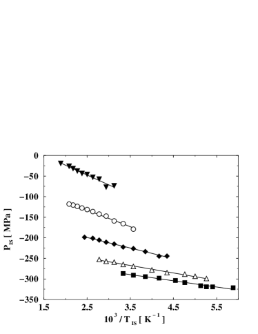
Figure 5: Inherent structure equation of state. Symbols are MD calculations, lines are PEL predictions.

Finally, Fig. 3 compares MD data (open symbols) and PEL (dashed lines) predictions in a run where $T$ is increased starting from the $T=0$ IS configuration, as previously discussed. The entire simulation is much shorter than the time needed to change basin, so that only the vibrational degrees of freedom are thermalized. Also in this case, the PEL expression accounts for the observed linear increase of $P$.

The present EOS, based exclusively on PEL properties, can and will be used to address important issues in the thermodynamics of supercooled liquids footnotebivariata , such as the study of the intrinsic limit of stability of the liquid state debenedettieos ; roberts ; sastry00 and the IS-based thermodynamic description of aging aging .

References

- (1) F. H. Stillinger, J. Phys. Chem. B 102, 2807 (1998).
- (2) R. J. Speedy, J. Chem. Phys. 110, 4559 (1999); J. Phys. Chem. B 103 , 4060 (1999); R. J. Speedy and P. G. Debenedetti, Mol. Phys. 88, 1293 (1996).
- (3) L. M. Martinez and C. A. Angell, Nature (London) 410, 667 (2001).
- (4) B. Coluzzi, P. Verrocchio, and G. Parisi, Phys. Rev. Lett. 84, 306 (2000); M. Mézard and G. Parisi, Phys. Rev. Lett. 82, 747 (1999).
- (5) D. J. Wales, Science 293, 2067 (2001).
- (6) P. G. Debenedetti and F. H. Stillinger, Nature (London) 410, 259 (2001).
- (7) F. Sciortino, W. Kob, and P. Tartaglia, Phys. Rev. Lett. 83, 3214 (1999).
- (8) S. Büchner and A. Heuer, Phys. Rev. E 60, 6507 (1999).
- (9) A. Scala et al., Nature (London) 406, 166 (2000).
- (10) S. Sastry, Nature (London) 409, 164 (2001).
- (11) I. Saika-Voivod et al. , Nature (London) 412, 514 (2001).
- (12) F. H. Stillinger and T. A. Weber, Phys. Rev. A 25, 978 (1982); Science 225, 983 (1984).
- (13) S. Mossa et al., Preprint cond-mat/0111519.
- (14) A. Heuer and S. Buchner, J. Phys.: Condens. Matter 12, 6535 (2000).
- (15) P. G. Debenedetti, F. H. Stillinger, T. M. Truskett, and C. J. Roberts, J. Phys. Chem. B 103, 7390 (1999).
- (16) F. Sciortino and P. Tartaglia, Phys. Rev. Lett. 86, 107 (2001).
- (17) E. La Nave et al., in preparation.
- (18) Note that liquids with non monotonic behavior of density (as water) must be characterized by a positive coefficient.
- (19) R. A. LaViolette, Phys. Rev. B, 40, 9952 (1989).
- (20) C. J. Roberts, P. G. Debenedetti, and F. H. Stillinger, J. Phys. Chem. B 103, 10258 (1999).
- (21) S. Sastry, P. G. Debenedetti, and F. H. Stillinger, Phys. Rev. E 56, 5533 (1997); S. Sastry, Phys. Rev. Lett. 85, 590 (2000).
- (22) G. Wahnström and L. J. Lewis, Phys. Rev. E 50, 3865 (1994).
- (23) Work is in progress lanave02 to elucidate the possibility that the dependence of the excess specific heat measured in constant experiments [C. Alba, L. E. Busse, D. J. List, and C. A. Angell, J. Chem. Phys. 92, 617 (1990)] can be understood using the PEL-EOS developed here.
- (24) Another interesting possibility is offered by a generalization to of Eq. (1). The oTP data allow us to eliminate the simple possibility that is a bivariate Gaussian lanave02 .