The breakdown of the shear modulus at the glass transition

U. Buchenau

Institut für Festkörperforschung, Forschungszentrum Jülich

Postfach 1913, D-52425 Jülich, Germany.

ABSTRACT

The glass transition is described in terms of thermally activated local structural rearrangements, the secondary relaxations of the glass phase. The interaction between these secondary relaxations leads to a much faster and much more dramatic breakdown of the shear modulus than without interaction, thus creating the impression of a separate primary process which in reality does not exist. The model gives a new view on the fragility and the stretching, two puzzling features of the glass transition.

The mode coupling theory of the glass transition (Götze and Sjögren 1992) postulates a crossover in the flow mechanism at the critical temperature $T_{c}$ to thermally activated hopping on the low-temperature side. This postulate has received strong support by recent simulations, which showed that the system passes from the saddle points of the energy landscape to the minima at exactly this critical temperature (for a review see Buchenau 2003). Thus one indeed expects thermally activated flow between $T_{c}$ and the calorimetric glass transition temperature $T_{g}$, where the system freezes.

However, if one looks at the temperature dependence of the flow process below $T_{c}$, it is dramatically faster than that of a thermally activated process, particularly for the so-called fragile glass formers (Böhmer et al 1993). This fragility seems to be linked to a strong stretching of the shear stress relaxation, extending over several decades in time. Both phenomena have not yet found a generally accepted explanation.

The present paper proposes to describe the glass transition in terms of the energy landscape concept (Goldstein 1968; Johari and Goldstein 1970, 1971; Stillinger 1995), taking the interaction between different thermally activated jumps into account. There is increasing evidence (Richert 2002) for a heterogeneous energy landscape dynamics. In the glass phase, the energy landscape idea has been successfully exploited in three phenomenological models, the tunneling model (Phillips 1981) for the glass anomalies below 1 K, the soft-potential model (Parshin 1994) for the crossover to higher temperatures and, finally, the ADWP (Asymmetric-Double-Well-Potential, Pollak and Pike 1972) or Gilroy-Phillips model (Gilroy and Phillips 1981) for the description of the classical relaxation over a wide range of barrier heights, up to barrier heights which become relevant for the flow process, i.e. barriers of the order of 35 $k_{B}T_{g}$.

As is well known, two relaxation centers at different positions interact via their elastic dipole moments. Here, it is proposed to treat this interaction in terms of the weakening of the shear modulus by the relaxation, a mean-field approach.

We describe the dynamical shear response of the glass or undercooled liquid in terms of the apparent barrier density function $f(V)$ defined by

$$\frac{\delta G}{G\delta V}\equiv f(V),$$ (1)

where $\delta G$ is the reduction of the shear modulus from all relaxations with barrier heights between $V$ and $V+\delta V$ and $G$ is the infinite frequency shear modulus. The relaxation time $\tau_{V}$ of these relaxation centers is given by the Arrhenius relation

$$\tau_{V}=\tau_{0}\exp(V/k_{B}T)$$ (2)

with $\tau_{0}\approx 10^{-13}s$.

One next needs the relation between the true barrier density $f_{0}(V)$ and the apparent density $f(V)$. Consider a constant shear strain $\epsilon_{0}$ applied at time $0$. The stress $\sigma$ after the time $t$ is given by

$$\sigma(t)=G(t)\epsilon_{0}=G\epsilon_{0}\int_{0}^{V_{M}}\exp(-t/\tau_{V})f(V)dV.$$ (3)

Here $V_{M}$ is the Maxwell barrier corresponding to the terminal relaxation time $\tau_{M}$ of the shear modulus, the Maxwell time.

A given relaxation center will tend to jump at its relaxation time $\tau_{V}$. At the time $\tau_{V}$, the stress is diminished by the factor $G_{V}/G$, where $G_{V}=G(\tau_{V})$. The local distortion at the center is assumed to be unchanged. This implies an unchanged contribution of the center to the free energy. Thus the reduction of the stress energy by the center is unchanged. But we reduce a smaller stress energy, so $f(V)$ must be larger than $f_{0}(V)$ by the square of the factor $G/G_{V}$. In a physical picture, the enhancement is due to induced jumps of lower-barrier entities in the neighbourhood, which reduce the resistance of the viscoelastic medium surrounding the center.

$G_{V}$ is given by

$$G_{V}=G\int_{0}^{V_{M}}\exp(-\tau_{V}/\tau_{v})f(v)dv\approx G\int_{V}^{V_{M}}f(v)dv,$$ (4)

because the double-exponential cutoff is practically a step function. Therefore it is reasonable to define the true barrier density function by

$$f_{0}(V)\equiv f(V)\left[\int_{V}^{V_{M}}f(v)dv\right]^{2},$$ (5)

since the integral on the right hand side is close to $G_{V}/G$.

Solving this integral equation for $f(V)$ one finds

$$f(V)=\frac{f_{0}(V)}{\left[3\int_{V}^{V_{M}}f_{0}(v)dv\right]^{2/3}}.$$ (6)

This solution has two important properties. The first is the 1/3-rule:

$$\int_{0}^{V_{M}}f_{0}(V)dV=\frac{1}{3}.$$ (7)

The rigidity vanishes when the integral over the noninteracting relaxation entities is 1/3, i.e. when the noninteracting secondary processes would have reduced the initial shear modulus at time zero to 2/3 of its value. The 1/3-rule has been derived independently from energy considerations (Buchenau 2003).

The second important property is that the breakdown occurs in a rather dramatic way, because the relaxing entities at the critical Maxwell barrier value receive a strong enhancement, to such an extent that one is tempted to assume a separate $\alpha$-process which has nothing to do with the secondary relaxations. In fact, this more or less unconscious assumption underlies most of the present attempts to understand the glass transition (Ediger, Angell and Nagel 1996). The above treatment shows such an assumption to be unnecessary; what one sees at the glass transition are simple Arrhenius relaxations of no particularly large number density, blown up to impressive size by the small denominator of eq. (6).

One can calculate the barrier density function from dynamical mechanical measurements in the glass phase using the approximation (Buchenau 2001)

$$f(V,T)\approx\frac{2}{\pi}\frac{G^{\prime\prime}}{Gk_{B}T},$$ (8)

where $V$ is calculated from the condition $\omega\tau_{V}=1$.

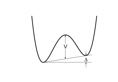
Figure 1: Asymmetric double-well potential.

Though the potential parameters freeze at $T_{g}$, $f_{0}(V,T)$ will still depend on temperature, even in the glass phase. This temperature dependence can be derived from a consideration on the free energy of an asymmetric double-well potential (Fig. 1). In the simplest possible approximation, the free energy of the relaxing entity is (Buchenau 2001)

$$F=-k_{B}T\ln\left[2\cosh\left(\frac{\Delta}{2k_{B}T}\right)\right].$$ (9)

The Boltzmann factor $\exp(-F/k_{B}T)$ at $T_{g}$ supplies the asymmetry distribution

$$P(\Delta)\sim\cosh(\Delta/2k_{B}T_{g}),$$ (10)

so the number density of relaxing entities does indeed increase with increasing $\Delta$; it is not really constant. If one integrates over the asymmetries at a lower temperature, one finds a diminution of the effective $f_{0}(V,T)$ by a factor of up to $\pi/2$ in the low temperature limit. A useful approximation below $T_{g}$ is

$$\frac{f(V,T_{g})}{f(V,T)}=\left[2{\rm arctan\ (e}^{V/2k_{B}T})-\frac{\pi}{2}\right]{\rm e}^{-(T_{g}/T)^{2}{\rm ln}(\pi/2)}$$ (11)

This factor has to be taken into account to calculate $f(V,T_{g})$ from measurements of the mechanical loss in the glass phase. Once $f(V)$ is known, $f_{0}(V)$ can be obtained from eq. (5).

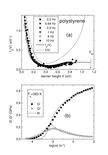
Figure 2: (a) $f_{0}(V,T_{g})$ for polystyrene from torsion pendulum data, together with the corresponding $f(V,T_{g})$ (b) measured and calculated dynamical shear data at the glass transition (references see text).

Fig. 2 (a) shows $f_{0}(V,T_{g})$ for polystyrene determined in this way from six torsion pendulum data at 0.5, 0.64, 0.9, 1, 6 and 10 Hz (Illers and Jenckel 1958; Schwarzl 1990a; Schmieder and Wolf 1953; Schwarzl 1990b; Sinnott 1959; Hartwig and Schwarz 1968). The data were fitted by the six-parameter expression

$$f_{0}(V,T_{g})=\frac{2C}{W^{3/4}V^{1/4}}{\rm e}^{-V/V_{0}}+a_{1}{\rm e}^{-g1(V-p1)^{2}}.$$ (12)

Two of the parameters, the energy $W$ and the small number $C$, can be taken from soft-potential fits of the low-temperature anomalies (Ramos and Buchenau 1997), because the first term is the barrier density of the soft-potential model (Parshin 1994), with an exponential cutoff of the soft-potential expectation at a limiting barrier $V_{0}$. The second term is just an appropriate gaussian with amplitude $a_{1}$ and width parameter $g_{1}$ centered at the position $p_{1}$. The results of the fit are compiled in Table I.

Table I: Fit parameters for $f_{0}(V,T_{g})$.

substance	$C$	$W$	$V_{0}$	$a_{1}$	$g_{1}$	$p_{1}$
	$10^{-4}$	$meV$	$eV$	$eV^{-1}$	$eV^{-2}$	$eV$
$a-SiO_{2}$	2.65	0.34	0.04	0.76	0.54	5.45
polystyrene	7.1	0.159	0.1	0.19	4.0	1.0

With these parameters, the integral over $f_{0}(V,T_{g})$ extrapolates to 1/3 at $V_{M}=1.1eV$, consistent with the experimental $T_{g}$ of 373 K, defining $T_{g}$ as the temperature where the terminal relaxation time $\tau_{t}$ reaches 100 s. This is the first time a glass temperature could be calculated from glass data alone (it is true that the glass temperature enters already in the calculation, but one can iterate, and the procedure converges quickly).

Even more impressive, the same parameter combination provides a very reasonable fit of the measured (Donth et al1996) $G^{\prime}(\omega)$ and $G^{\prime\prime}(\omega)$ at the glass temperature (for this sample at 363 K). This is shown in Fig. 2 (b), calculated with $G=1.55$ GPa, the value obtained from the Brillouin transverse sound velocity (Strube, private communication) of 1071 m/s, taking the weakening by $f_{0}(V)$ at the Brillouin frequency into account. The sharp barrier cutoff at $V_{M}$ of the model seems to be too sharp for this polymer case, possibly because of the crossover from enthalpic to entropic restoring forces.

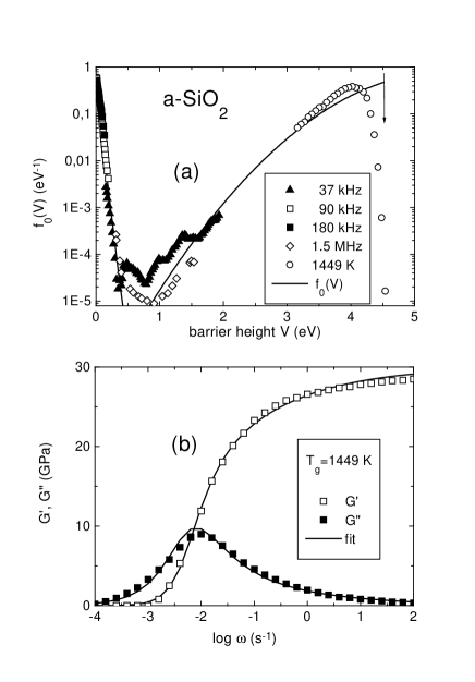
Figure 3: (a) $f_{0}(V,T_{g})$ for $SiO_{2}$ from measurements at four frequencies and from the dynamical glass transition data (b) measured and calculated dynamical shear data at the glass transition (references see text).

Fig. 3 (a) shows the barrier density function in the strong glass former $SiO_{2}$. From measurements at 90 and 180 kHz (Cahill and van Cleve 1989; Keil, Kasper and Hunklinger 1993), one finds again the soft-potential model expectation $f_{0}(V,T_{g})=2C/W^{3/4}V^{1/4}$ at very low barriers, with $C$ and $W$ taken from fits to the low-temperature thermal conductivity and specific heat (Ramos and Buchenau 1997). There is a pronounced exponential cutoff over more than four decades leading to very low mechanical damping at and above room temperature, the lowest observed in any glass so far. Data close to $T_{g}$ are rather scarce. Therefore it turned out to be necessary to include the data (Mills 1974) for $G^{\prime}(\omega)$ and $G^{\prime\prime}(\omega)$ at $T_{g}$ into the fit for the high-barrier gaussian in eq. (12). Thus, one cannot predict $T_{g}$ from glass phase data alone as in polystyrene. The fulfillment of the 1/3-rule required $G=30.2$ GPa for the fit of Fig. 3 (b), while transverse wave Brillouin data (Bucaro and Dardy 1974) suggest a value of $33.7$ GPa. Nevertheless, having fitted $f_{0}(V)$ both at the low- and high-barrier end, it is gratifying to see the good agreement of the very low damping at and above room temperature for 37 kHz (Marx and Sivertsen 1953) and 1.5 MHz (Fraser 1970) in Fig. 3 (a), because these data were not used to obtain the fit. Also, Fig. 3 (b) shows that in this case the sharp cutoff gives a much better fit of the stretching than in polystyrene.

Note that not all glass formers can be fitted by the simple form of eq. (12); many glass formers show several separate secondary relaxation peaks.

Finally, let us turn to the fit of the fragility. This requires the temperature dependence of a whole function, namely $f_{0}(V,T)$ above $T_{g}$. Here, the estimate for this dependence is based on the Boltzmann factor of eq. (10). Obviously, the rise of the Boltzmann factor with increasing asymmetry $\Delta$ cannot go on forever. We assume that it stops at $\Delta=b_{o}V$, where $b_{o}$ is a fit parameter of order 1. One expects a return to a kind of low-energy glass ground state when the asymmetry gets as large as the barrier height.

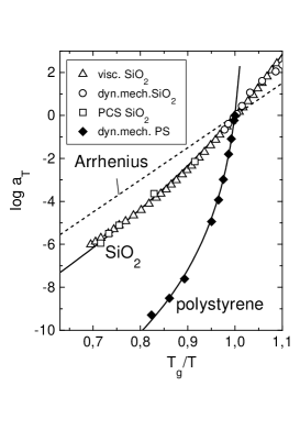
Figure 4: Angell plot for polystyrene and $SiO_{2}$. The dashed line shows the Arrhenius law, the continuous lines the model fits explained in the text.

This assumption allows to calculate a partition function for a given barrier height. From this partition function, $f_{0}(V,T)$ should follow the equation

$$\frac{f_{0}(V,T)}{f_{0}(V,T_{g})}=\frac{T_{g}}{T}\frac{{\rm sinh}(b_{o}V/2k_{B}T_{g})}{{\rm sinh}(b_{o}V/2k_{B}T)}$$ (13)

for temperatures above $T_{g}$.

With this equation, one can calculate the shift factor $a_{T}=\tau_{M}(T)/\tau_{M}(T_{g})$ from the 1/3-rule, eq. (7). The result is compared in Fig. 4 to measurements (Mills 1974; Bucaro and Dardy 1977; Plazek and O’Rourke 1971). The fit parameter $b_{o}$ was 1.4 for polystyrene and 0.33 for silica. The difference in fragility does not only stem from this difference, but also from the large difference in $f_{0}(V_{M})$ at $T_{g}$: a rise in the number of relaxing entities shifts the Maxwell barrier much farther in polystyrene than in silica.

This fragility fit may be too simple-minded, but it points the way to a new understanding. If $f_{0}(V,T)$ increases with increasing temperature, the Maxwell barrier will decrease. Once one accepts the idea of a relatively high free energy of a symmetric double-well potential in the undercooled liquid, the fragility ceases to be a puzzling property.

References

References

- [1] [] Böhmer R., Ngai K. L., Angell C. A. and Plazek D. J. 1993 J. Chem. Phys. 99 4201
- [2] [] Bucaro J. A. and Dardy H. D. 1974 J. Appl. Phys. 45, 5324
- [3] [] Bucaro J. A. and Dardy H. D. 1977 J. Non-Crystalline Solids 24, 121
- [4] [] Buchenau U. 2001 Phys. Rev. B 63, 104203
- [5] [] Buchenau U. 2003 preprint cond-mat/0209172, Energy landscape - a key concept in the dynamics of liquids and glasses; J. Phys.: Condens. Matter 15, S955
- [6] [] Cahill D. G. and van Cleve J. E. 1989 Rev. Sci. Instrum. 60, 2706
- [7] [] Donth E., Beiner M., Reissig S., Korus J., Garwe F., Vieweg S., Kahle S., Hempel E. and Schröter K. 1996 Macromolecules 29, 6589-6600
- [8] [] Fraser D. B. 1970, J. Appl. Phys. 41, 6
- [9] [] Geis N., Kasper G. and Hunklinger S. 1986, in Non-metallic Materials and Composites at Low Temperatures 3, ed. by Hartwig G. and Evans D., p. 99 (Plenum Press, New York)
- [10] [] Gilroy K. S. and Phillips W. A. 1981 Phil. Mag. B 43, 735
- [11] [] Götze W. and Sjögren L. 1992 Rep. Prog. Phys. 55 241
- [12] [] Goldstein M. 1968 J. Chem. Phys. 51, 3728
- [13] []Hartwig G. and Schwarz G. 1986, in Nonmetallic Materials and Composites at Low Temperatures 3, ed. by Hartwig G. and Evans D., p. 117 (Plenum Press, New York)
- [14] [] Illers K. H. and Jenckel E. 1958 Rheol. Acta 1, 322
- [15] [] Keil R., Kasper G. and Hunklinger S. 1993 it J. Non-Cryst. Sol. 164-166, 1183
- [16] [] Johari G. P. and Goldstein M. 1970 J. Chem. Phys. 53 2372
- [17] [] Johari G. P. and Goldstein M. 1971 J. Chem. Phys. 55 4245
- [18] [] Marx J. W. and Sivertsen J. M. 1953 J. Appl. Phys. 24, 81
- [19] [] Mills J. J. 1974 J. Noncryst. Solids 14, 255
- [20] [] Parshin, D. A. 1994 Phys. Solid State 36, 991
- [21] [] Phillips, W. A. (ed.) 1981, Amorphous Solids: Low temperature properties, (Springer, Berlin)
- [22] [] Plazek D. J. and O’Rourke V. M. 1974 J. Polym. Sci: Part A-2 9, 209
- [23] [] Pollak M. and Pike G. E. 1972 Phys. Rev. Lett. 28 1449
- [24] [] Ramos, M. A., and Buchenau, U. 1997 Phys. Rev. B 55, 5749
- [25] [] Richert R. 2002 J. Phys.: Condens. Matter 14 R703-R738
- [26] [] Schmieder K. and Wolf K. 1953 Kolloid-Z. 136, 157
- [27] [] Schwarzl F. R. 1990a Polymermechanik (Springer, New York), Fig. 5.16
- [28] [] Schwarzl F. R. 1990b Polymermechanik (Springer, New York), Fig. 6.12
- [29] [] Sinnott K. M. 1959 J. Polym. Sci. 128, 273