Interaction-driven effects on two-component Bose-Einstein condensates

Abstract

We investigate the role of the interparticle-interaction strength in the distribution of two species of atoms inside a condensate. We focus upon the study of systems for which the minima of the trapping potentials for the species are displaced from each other by a distance that is small compared to the size of the total condensate. We show that in a small range of the interparticle-interaction strength the distribution of species undergoes dramatic changes, and exhibits a variety of different features. We demonstrate that this behavior can be easily understood in terms of the Thomas-Fermi approximation. This effect may be useful in experimentally determining the values of the scattering lengths.

Much experimental and theoretical work in Bose-Einstein Condensation deals with systems composed of a mixture of two distinct species of atoms fe01 ; ma98 ; ma99 ; an00 ; an01 ; ha98 . For example, one mixture commonly used is that of atoms of ⁸⁷Rb in two different hyperfine states $|F=1,m_{f}=-1\rangle$ and $|F=2,m_{f}=1\rangle$ ma98 . This mixture has shown itself to be very useful for experimentally generate topological modes, such as different types of vortices ma99 ; an00 ; an01 . Experimentally these mixtures are under conditions such that the species behave as “effectively distinguishable”, and have been observed to separate partially in space ha98 . An interesting issue to investigate is how the particles distribute themselves inside the condensate depending on the interparticle interaction, specially because there still exists uncertainty about its numerical value.

From a theoretical point of view, H. Pu and N. P. Bigelow studied the ground state properties of different mixtures in a spherically symmetric trapping potential. In Ref. pu98 , they displayed the density profiles of both components for various combinations of scattering lengths below phase separation, testing the validity of the Thomas- Fermi approximation. Later, E. Timmermans extended the study to phase separation ti98 . In particular he showed that in a spherically symmetric trap the less repulsive component remains inside a sphere while the other component lies in a spherical shell around it.

In this work we analyze the case when one of the species is in a slightly shifted potential with respect to the other species, and thus the spherical symmetry is broken. We find that by varying the interparticle interaction strength by less than $10$%, the particles rearrange themselves in very different configurations inside the condensate. As far as we know, this problem was only studied for a particular set of scattering lengths es97 and it still lacks an easy interpretation. Here we show that the distribution of species can be easily understood in terms of the Thomas-Fermi (TF) approximation. We compute the exact Gross-Pitaevskii (GP) solutions for a large number of particles and find that TF predictions describe with great accuracy the geometrical properties of the distribution of species within the condensate.

In order to describe the wave functions of two-species condensates one has to solve the coupled Gross-Pitaevskii equations da99 :

$$\left(-\frac{\hbar^{2}\nabla^{2}}{2M_{i}}+V_{i}+N_{i}G_{i,i}|\Psi_{i}|^{2}\right. + \left.\sum_{k}N_{k}G_{i,k}|\Psi_{k}|^{2}\right)\,\Psi_{i}$$ (1)

$$= \mu_{i}\Psi_{i}.$$

where $N_{i}$ and $M_{i}$ denote the number of atoms and the mass of the species $i$, respectively. The factors $G_{k,l}=u_{k,l}U$, with $u_{k,l}$ being the relative interaction strengths between species $k$ and $l$, and $V_{i}$ the potential seen by species $i$. Hereafter, we consider a two component system and set the most repulsive component $|1\rangle$ in the $\Psi_{1}$ state, fixing $u_{1,1}=1$ $(>u_{2,2})$, so $U=4\pi\hbar^{2}a/M_{1}$, $a$ being the scattering length of the $|1\rangle$-species. In addition, for simplicity, we set $M_{1}=M_{2}=M$.

Qualitative analysis—

In order to study qualitatively how the species rearrange themselves inside the condensate when varying the relative interparticle strength $u_{1,2}$, we make use of the Thomas Fermi (TF) approximation, which consists of neglecting the kinetic energy, and thus removing the laplacian terms in Eqs. (1). We will consider a system in which both components are in an axially symmetric trap and the $|2\rangle$ component has the minimum shifted in the $z$ direction by a value $-d$. We make a change of variables according to $\sqrt{(M/2)}\omega_{z}\vec{r}\rightarrow\vec{r}$, where $\omega_{r}$ and $\omega_{z}$ are the trap angular frequencies in the $r$ and $z$ coordinate, respectively. Futhermore, by defining the aspect ratio $\lambda=\omega_{r}/\omega_{z}$, the potentials $V_{i}$, written in cylindrical variables, read

$$V_{1}=\lambda^{2}r^{2}+z^{2}$$ (2)

and

$$V_{2}=\lambda^{2}r^{2}+(z+d)^{2}.$$ (3)

The sign of the determinant $\Delta\equiv u_{1,1}u_{2,2}-u_{1,2}^{2}$ defines two different features for the distribution of particles. When $\Delta>0$ and $u_{1,2}$ is small, there exists a large coexistence region. As $u_{1,2}$ is increased this region decreases. At $\Delta=0$, a phase separation takes place reducing the coexistence region to an interface. We shall consider the cases $\Delta>0$ and $\Delta<0$ separately.

Coexistence $\Delta>0$—

The solution of Eqs. (1) in the TF approximation can be easily obtained and has the following different expressions depending on whether there exists any overlap between the wave functions of both species.

a) In the region where only one wave function is non vanishing ( $|\Psi_{i}|^{2}\neq 0$ and $|\Psi_{k}|^{2}=0$, for $i\neq k$) the TF equations are decoupled and the solution reads

$$|\Psi_{1}|^{2} = \left[\mu_{1}-\lambda^{2}r^{2}-z^{2}\right]/(G_{1,1}N_{1}),$$

$$|\Psi_{2}|^{2} = \left[\mu_{2}-\lambda^{2}r^{2}-(z+d)^{2}\right]/(G_{2,2}N_{2}).$$ (4)

b) In the region where both wave functions are non vanishing $|\Psi_{i}|^{2}>0$, the solution may be written after some algebra as:

$$|\Psi_{1}|^{2} = \left[R_{1}^{2}-\lambda^{2}r^{2}-\left(z-\frac{\beta_{1}d}{1-\beta_{1}}\right)^{2}\right]B_{1}\,u_{2,2},$$

$$|\Psi_{2}|^{2} = \left[R_{2}^{2}-\lambda^{2}r^{2}-\left(z+\frac{d}{1-\beta_{2}}\right)^{2}\right]B_{2}\,u_{1,1},$$ (5)

with

$$R_{1}^{2} = \frac{\mu_{1}-\beta_{1}\mu_{2}}{(1-\beta_{1})}+\frac{\beta_{1}d^{2}}{(1-\beta_{1})^{2}},$$

$$R_{2}^{2} = \frac{\mu_{2}-\beta_{2}\mu_{1}}{(1-\beta_{2})}+\frac{\beta_{2}d^{2}}{(1-\beta_{2})^{2}},$$ (6)

where $\beta_{1}=u_{1,2}/u_{2,2}$, $\beta_{2}=u_{1,2}/u_{1,1}$ and $B_{i}=(1-\beta_{i})/(UN_{i}\Delta)$.

The surfaces $\cal{S}$₁ and $\cal{S}$₂, defined by equating the expression inside the square bracket in $|\Psi_{1}|^{2}$ and $|\Psi_{2}|^{2}$ of Eq. (5) respectively to zero, determine the boundary of the coexistence region. It may be seen that these surfaces are ellipsoids centered in $d_{1}=\beta_{1}d/(1-\beta_{1})$ and $d_{2}=-d/(1-\beta_{2})$ along the $z$-axis, respectively. It is worth mentioning that this result does not depend on any other quantity, as for example the number of particles or the frequencies of the trapping potential. The factor $1-\beta_{i}$ in the denominator makes these displacements diverge when $\beta_{i}$ is close to unity, and one can guess that for these values, some dramatic effects in the redistribution of particles could take place, as we shall discuss later.

Phase separation $\Delta<0$ —

For these interaction strengths, in the Thomas-Fermi approximation, the species are confined to two separated regions within the condensate. The boundary surface $\cal{S}$_s between these two regions may be obtained by equating the pressure da99

$$P_{i}=\frac{G_{i,i}}{2}|\Psi_{i}|^{4}$$ (7)

on both sides of the interface, yielding

$$|\Psi_{1}|^{2}=\sqrt{\frac{G_{2,2}}{G_{1,1}}}|\Psi_{2}|^{2}.$$ (8)

Assuming that the wave functions on each side are given by the expression (4) and defining $a=\sqrt{G_{2,2}/G_{1,1}}$, the interface obtained is

$$R_{s}^{2}-\lambda^{2}r^{2}-\left(z+\frac{d}{1-a}\right)^{2}=0$$ (9)

with

$$R_{s}^{2}=\frac{\mu_{2}-a\mu_{1}}{(1-a)}+\frac{ad^{2}}{(1-a)^{2}}.$$ (10)

This surface is an ellipsoid whose center is displaced in $d_{s}=-d/(1-a)$ along the $z$-axis. Note that the quantities $R_{s}$ and $d_{s}$ do not depends on $u_{1,2}$. It is easy to prove that for $\Delta=0$ the surfaces verify $\cal{S}$${}_{1}\equiv\cal{S}$${}_{2}\equiv\cal{S}$_s.

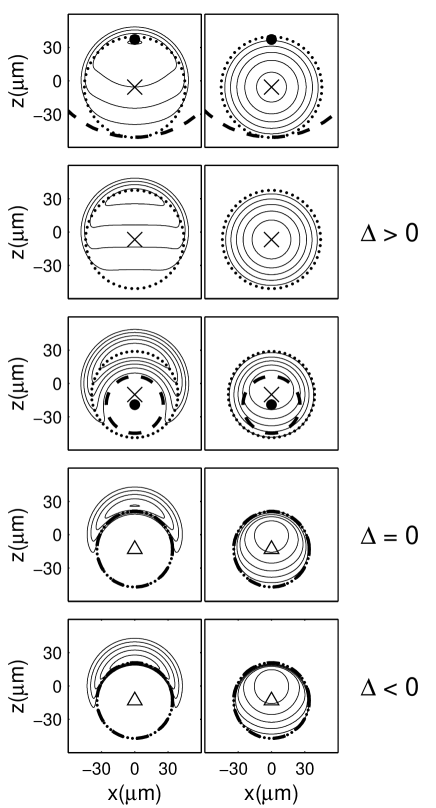
Figure 1: GP density contours of $\rho_{1}$ and $\rho_{2}$ are shown in the first and second column, respectively. From top to bottom of the graph, the rows correspond to relative interparticle interaction strengths $u_{1,2}$ = $0.93$, $0.94$, $0.96$, $\sqrt{0.94}$ and $1$. The dashed, dotted and dash-dotted lines correspond to TF radii $R_{1}$, $R_{2}$, and $R_{s}$, respectively. The dot, cross and triangle indicate $d_{1}$, $d_{2}$, and $d_{s}$, respectively. The trapping potential displacement is $d=0.4\mu$m.

In what follows we consider only $\lambda=1$ in which case the surfaces $\cal{S}$_i are spheres with radii $R_{i}$.

In the TF approximation, the density contours $\rho_{i}=|\Psi_{i}|^{2}$ $(i=1,2)$ inside the coexistence region are spherical surfaces with radii $R<R_{i}$ ( $R>R_{i}$) if $\beta_{i}<1$ ($\beta_{i}>1$) centered in $d_{i}$.

Numerical results—

On the one hand, we compute the displacements $d_{i}$ and radii $R_{i}$ in the Thomas-Fermi approximation. Note that these radii depend on the chemical potentials, and thus also on both the number of particles and the trap frequencies. On the other hand, in order to obtain the exact densities, we solved the Gross-Pitaevskii equations, using a steepest descent method.

In particular, we used the relative intraparticle interaction strength of atoms of ⁸⁷Rb in the two different hyperfine states given, within a $1.2$% of error, in Ref. ma98 , $u_{1,1}=1$ and $u_{2,2}=0.94$. We chose a trapping potential with an angular frequency $\omega_{r}=2\pi\times 7.8$ Hz, and set the number of particles of each species $N_{1}=N_{2}=1$$\times$$10^{7}$.

In Fig. 1 we show the Gross-Pitaevskii density contours $\rho_{i}$ in the $y=0$ plane, together with the Thomas-Fermi displacements $d_{i}$ and radii $R_{i}$, for $d=0.4$ $\mu$m. From the first to the last row we vary $u_{1,2}$ by less than $10$%. For $u_{1,2}=0.93$, which corresponds to the first row of the graph, it can be seen that a large coexistence region still exists. This region is given by the intersection of the circles defined by $R_{i}$ and $d_{i}$, which leaves outside only a little region on the top of the condensate filled with $|1\rangle$ type particles. It can also be seen that inside the coexistence region, the GP density contours are well-described by spherical surfaces centered in the points $d_{1}$ and $d_{2}$ for $\rho_{1}$ and $\rho_{2}$ respectively, as predicted with the TF approximation. For the second row we consider $u_{1,2}=0.94$, and with this value $d_{1}$ and $R_{1}$ diverge. The density contours inside the coexistence region are quite planar surfaces for the $|1\rangle$ component, as expected from the TF analysis because of the above-mentioned divergences. For $u_{1,2}=0.96$, which is displayed in the third row, three phases already exist: pure $|1\rangle$ and $|2\rangle$ components and a coexistence region. Once more, the contours seem to be in agreement with formulae (4) and (5) with only a small departure in the region next to the boundaries.

Phase separation occurs for $u_{1,2}=\sqrt{0.94}$, which corresponds to the fourth row, and thus the coexistence region is reduced to a surface. It is evident that although the GP solutions exhibit some overlap the general feature of the condensate is well-described by the TF approximation. Of course, if we take a smaller number of particles into account, the overlap will be greater. The last row corresponds to $u_{1,2}=1$ which is quite similar to the previous figure. This is due to the fact that formulae (9) and (10) do not depend on $u_{1,2}$, as we stated before.

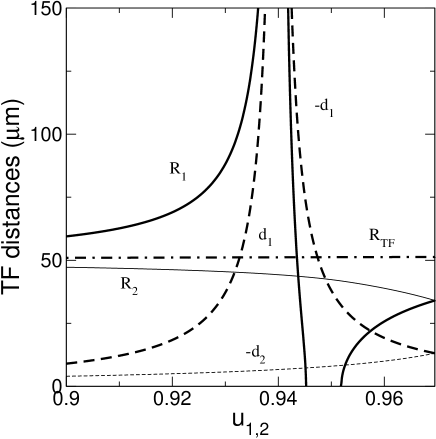
Figure 2: Thomas-Fermi displacements $|d_{1}|$ (thick dashed line), $|d_{2}|$ (thin dashed line), radii $R_{1}$ (thick solid line) and $R_{2}$ (thin solid line), and the TF radius of the condensate $R_{\text{TF}}$ (dash-dotted line) as function of the interparticle interaction strength $u_{1,2}$ for the same conditions as in Fig. 1.

In Fig. 2 we display the TF quantities, $d_{i}$ and $R_{i}$ together with the radius of the condensate $R_{\text{TF}}$ as functions of $u_{1,2}$. For $u_{1,2}<0.9$, all these quantities are smooth and monotonous functions, while in the interval displayed in the figure, the quantities related to $|1\rangle$ species exhibit an abrupt behavior. This effect suggests that if one wants to test experimentally the validity of the values of the interaction strengths within this interval by determining the displacements $d_{i}$, the error in their determination should not affect the desired quantities too much.

As a final illustration, in Fig. 3 we display the density contour for two different sets of relative scattering lengths to describe the interaction of the same two species of ⁸⁷Rb. One set, which is assumed to be more accurate ha98 , is $u_{1,1}=1,u_{1,2}=0.97$ and $u_{2,2}=0.94$. However, to tell the truth, up to our knowledge, the error of $u_{1,2}$ is not given anywhere. For these values of the interaction strengths the determinant is negative ($\Delta=-9$$\times$$10^{-4}$) and thus the system is phase separated, and hence the coexistence region in the Thomas Fermi approximation is reduced to an interface. The other, previously used, set of parameters es97 is $u_{1,1}=1,u_{1,2}=108/109$ and $u_{2,2}=108.8/109$, and verifies $\Delta=1.6$$\times$$10^{-2}$. Since the determinant is positive a coexistence region exists. Moreover, $\beta_{1}=0.99$ is less than $1$, and the contours of the $|1\rangle$ component at the coexistence region are still concave upwards.

We used three different displacements $d=0.4,1,1.5$ $\mu$m for the trapping potentials. For the first set of interaction strengths the corresponding TF displacements are $d_{s}=-13,-32,-49$ $\mu$m, respectively. While for the second set, the displacements are $d_{1}=54,135,202$ $\mu$m and $d_{2}=-44,-109,-163$ $\mu$m. It may be seen that the distribution of particles is very different in both cases, especially for small displacements, and this fact can be used for testing experimentally the values of the scattering lengths. It is worth mentioning that in the experimental conditions of Ref. ha98 , as they obtain integrated densities, one cannot distinguish between a phase separated system ($\Delta<0$) and a system in which the components are overlapped ($\Delta>0$).

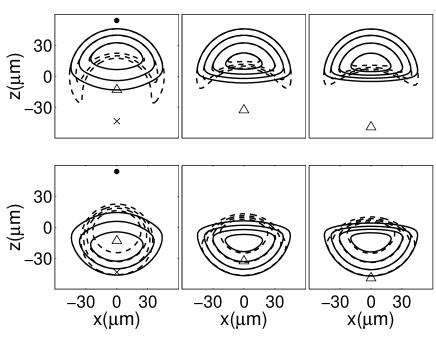
Figure 3: The first and second row show the GP density contours of $\rho_{1}$ and $\rho_{2}$, respectively. From the first to the third column we consider $d=0.4$, $1$, and $1.5$ $\mu$m. The dashed lines correspond to the set $u_{1,1}=1,u_{1,2}=0.97$ and $u_{2,2}=0.94$ while the solid lines correspond to the relative interaction strengths $u_{1,1}=1,u_{1,2}=108/109$ and $u_{2,2}=108.8/109$. The TF points $d_{s}$ (for the first set of parameters), and $d_{1}$ and $d_{2}$ are marked with a triangle, a dot and a cross, respectively.

Finally, having in mind the relations $\beta_{1}=d_{1}/(d+d_{1})$ and $\beta_{2}=(d+d_{2})/d_{2}$, we wondered wether having the experimental density contours in a given plane, say $y=0$, one can accurately determine the scattering lengths (see definitions of $\beta_{i}$) by estimating the displacements $d_{i}$. In order to answer this question we have done the following test. We have used the information of the GP density contours assuming that they represent the exact experimental data. For a given density contour $z(x)$ in the $y=0$ plane we computed the slope $b=\partial z/\partial x$ at each point $(x,z)$ of the curve. Then we calculated the intersection point between the line perpendicular to the density contour and $x=0$, which gives the center of the spherical surface. This point is $z_{c}=z+x/b$. Plotting $z_{c}$ for points all over the $|1\rangle$ ($|2\rangle$) component contour we found well-defined plateaus at $z_{c}=0$ ( $z_{c}=-d$) for points outside the coexistence region, and in $z_{c}=d^{*}_{1}$ ( $z_{c}=d^{*}_{2}$), where $d^{*}_{i}$ are the estimates of the TF $d_{i}$. We used this information to determine the scattering lengths and found an error in their determination of about $0.1$%. Note that, even considering an error in $z_{c}$ of about 30 $\mu$m and using the expressions of $\beta_{i}$, the uncertainty in the value of $u_{1,2}$ turns out to be below 0.5%. A similar procedure could be carried out with experimental data.

In summary, we show that the distribution of components is strongly ruled by the interparticle interaction strength, and for the number of particles we have considered, the way the particles rearrange inside the condensate can be easily understood in terms of the Thomas-Fermi approximation. We also outline a possible procedure to experimentally determine the relative scattering lengths.

References

- (1) A. L. Fetter and A. A. Svidzinsky, J. Phys.: Condens. Matter 13, R135 (2001); Tin-Lun Ho and V. B. Shenoy, Phys. Rev. Lett. 77 3276 (1996); P. Ohberg and S. Stenholm, Phys. Rev. A 57, 1272 (1998); D. Gordon and C. M. Savage, Phys. Rev. A 58, 1440 (1998); D. M. Jezek, P. Capuzzi, and H. M. Cataldo, Phys. Rev. A 64, 023605 (2001).
- (2) M. R. Matthews, D. S. Hall, D. S. Jin, J. R. Ensher, C. E. Wieman, E. A. Cornell, F. Dalfovo, C. Minniti, and S. Stringari, Phys. Rev. Lett. 81, 243 (1998).
- (3) M. R. Matthews, B. P. Anderson, P. C. Haljan, D. S. Hall, C. E. Wieman, and E. A. Cornell, Phys. Rev. Lett. 83, 2498 (1999).
- (4) B. P. Anderson, P. C. Haljan, C. E. Wieman, and E. A. Cornell, Phys. Rev. Lett. 85, 2857 (2000).
- (5) B. P. Anderson, P. C. Haljan, C. A. Regal, D. L. Feder, L. A. Collins, C. W. Clark, and E. A. Cornell, Phys. Rev. Lett. 86, 2926 (2001).
- (6) D. S. Hall, M. R. Matthews, J. R. Ensher, C. E. Wieman, and E. A. Cornell, Phys. Rev. Lett. 81, 1539 (1998).
- (7) H. Pu and N. P. Bigelow, Phys. Rev. Lett. 80, 1130 (1998).
- (8) E. Timmermans, Phys. Rev. Lett. 81, 5718 (1998).
- (9) B. D. Esry, Chris H. Greene, James P. Burke, and John L. Bohn, Phys. Rev. Lett. 78, 3594 (1997).
- (10) F. Dalfovo, S. Giorgini, L. Pitaevskii, and S. Stringari, Rev. Mod. Phys. 71, 463 (1999).