Independent neurons representing a finite set of stimuli: dependence of the mutual information on the number of units sampled

Abstract

We study the capacity with which a system of independent neuron-like units represents a given set of stimuli. We assume that each neuron provides a fixed amount of information, and that the information provided by different neurons has a random overlap. We derive analytically the dependence of the mutual information between the set of stimuli and the neural responses on the number of units sampled. For a large set of stimuli, the mutual information rises linearly with the number of neurons, and later saturates exponentially at its maximum value.

1 Experimental measures of redundancy

The capacity with which a population of neurons, or neuron-like units, can represent a set of elements in the outside world is an important issue both for experimental studies of neural coding and for theoretical analysis of neural network models. In the former situation, typically a discrete set of $p$ stimuli is presented to a subject while the activity of a population of $N$ neurons is recorded. The measured response can be represented as an $N$ dimensional vector ${\bf r}$, whose components stand for the activity of individual neurons, computed over a predefined time window. This activity is expected to be selective, at least to some degree, to each one of the stimuli. The degree of selectivity can be quantified by the mutual information between the set of stimuli and the responses (Shannon 1948)

$$I=\sum_{s=1}^{p}P(s)\sum_{{\bf r}}P({\bf r}|s)\ \log_{2}\left[\frac{P({\bf r}|s)}{P({\bf r})}\right],$$ (1)

where $P(s)$ is the probability of showing stimulus $s$, $P({\bf r}|s)$ is the conditional probability of observing response ${\bf r}$ when the stimulus $s$ is presented and

$$P({\bf r})=\sum_{s=1}^{p}P(s)\ P({\bf r}|s).$$ (2)

The mutual information $I$ characterizes the mapping between the $p$ stimuli and the response space, and represents the amount of information conveyed by ${\bf r}$ about which of the $p$ elements was shown.

If each of the stimuli evokes a unique set of responses, i.e. the responses are different for different stimuli, then Eq. (1) reduces to the entropy of the set of stimuli $H\{s\}=-\sum_{s}P(s)\log_{2}P(s)$. When the stimuli are equiprobable, the subject is exposed to the most variable presentation of the $p$ elements, and the entropy of the stimuli reaches its maximum value, that is, $\log_{2}(p)$. For other choices of $P(s)$, the mutual information is still bounded by $H\{s\}$, which in turn, is less than $\log_{2}p$.

On the other hand, if a response ${\bf r}$ may be evoked by more than one stimulus, the mutual information is less than $H\{s\}$. In the extreme case where the responses are independent of the stimuli, $I=0$. In short, the mutual information quantifies how precisely can any single stimulus be identified out of the $p$ possible ones, by measuring the response of the $N$ units.

Here, we are interested in describing the dependence of the mutual information with the number of neurons sampled. Such a dependence is crucial in quantifying the redundancy between the messages carried by different cells. Since information is an additive quantity, if different neurons provide independent information, we expect $I(N)$ to grow linearly with $N$. In fact, any departure of linearity is a sign of either a redundant or a synergetic coding (depending on whether the behaviour is sub or supra-linear). However, before drawing conclusions about the way information is shared among the neurons, it is important to understand to what extent the experimental design, more precisely, the set of stimuli chosen, determines by itself the shape of $I(N)$. As stated above, the maximum information that can be extracted from the neural responses is $H\{s\}$. It is clear that if we have a set of neurons that already provides an information very near to this maximum, by adding one more unit we will gain no more than redundant information. In other words, we have reached a regime where the neural responses correctly identify all of the stimuli. But we cannot deduce from this that the representational capacity of the responses remains unchanged when the number of neurons increases. One should rather realize that the task itself is no longer appropriate to test the way additional neurons contribute in the encoding of the stimuli.

Gawne and Richmond (1993) have considered this issue quantitatively, when recording from pairs of neurons. They presented a simple model which yields an analytical expression for $I(N)$ under the assumption that each neuron provides a fixed amount of information $I(1)$, and that a fixed fraction $y$ of such an amount is redundant with the information conveyed by any other neuron. In figure 1

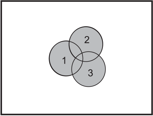
Figure 1: Schematic representation of Gawne and Richmond’s process (1993). The area of each circle represents the amount of information $I(1)$ provided by a single neuron. Different circles correspond to different neurons. Any two pair of neurons share an overlap $yI(1)$.

we reproduce their scheme, where all pairs of neurons are supposed to share the same redundancy $yI(1)$. Their model yields

$$I(N)=\frac{I(1)}{y}\left[1-(1-y)^{N}\right].$$ (3)

Here, $I(1)$ and $y$ are considered independent quantities. Gawne and Richmond (1993) measured both of them, using a single electrode to record the activity of pairs of nearby neurons. They got an average value for $I(1)=0.23$ bits, and their mean redundancy $y=[2I(1)-I(2)]/I(1)=0.2$. According to equation (3), as $N$ increases, $I(N)$ approaches a limiting value equal to $I(1)/y$. In their formulation, no attention is payed to the fact that $I(\infty)$ should approach $H\{s\}$, at least if the subject is behaviourally able to identify every single stimulus. According to the measured values of $y$ and $I(1)$, Gawne and Richmond calculated $I(\infty)=1.15$. Since in their case $H\{s\}=\log_{2}p=5$, they concluded that the assumption that all pairs of neurons share the same amount of redundant information, as measured by nearby neurons, was wrong.

What appeared important, then, was to go beyond what could be extrapolated from the shared information between pairs of cells, and measure directly the information that could be extracted from large populations. From the experimental point of view, this meant to measure the activity of a large number of units, ideally, with simultaneous recordings. Rolls et al(1997) have performed the experiment measuring the responses from cells in the inferior temporal cortex of a macaque, when exposed to $p$ visual stimuli. They recorded one neuron at a time, and therefore, were not able to capture the correlations in the neural responses present in every single trial. One should bear in mind, however, that such non-simultaneous recordings correctly describe the information carried by the firing rates of the neurons, and are exact in the limit of short time windows (Panzeri et al, 1999a).

In figure 2

Figure 2: Mutual information extracted from neural responses from the inferior temporal cortex of a macaque when exposed to $p$ visual stimuli (from Rolls et al1997). Diamonds correspond to $p=20$, squares to $p=9$ and triangles to $p=4$. The graph is plotted as a function of the neurons considered. We see that initially the information grows linearly, and eventually slows down For $p=4$, the curves clearly saturate at $\log_{2}p=2$.

we show their estimation of $I(N)$, after a decoding procedure. In their experiment, stimuli were equiprobable, so $H\{s\}=\log_{2}p$. Diamonds correspond to $p=20$, squares to $p=9$ and triangles to $p=4$. The graph is plotted as a function of the number of neurons sampled. Each line is an average of all the possible curves that could be made, depending on the order in which the neurons are selected. We see that initially the information grows linearly, and later descelerates. For $p=4$ there is a clear saturation at $\log_{2}4=2$ bits. For $p=9$ and $p=20$ the behaviour of the curves is compatible with the predicted asimptotes, at $\log_{2}9\approx 3,16$ bits and $\log_{2}20\approx 4,23$ bits. This experiment shows that the pool of neurons sampled appears to reach the entropy of the set of stimuli, showing that the activity of a sufficiently large number of cells carries the information needed to correctly identify every single element.

In order to explain their results, Rolls et alhave considered a more constrained model than the one of Gawne and Richmond, that further assumes that $y=I(1)/\log_{2}p$. This means that the only parameter to be measured is now $I(1)$. Their approach also leads to equation (3), but now $I(\infty)=\log_{2}p$. A fit of their expression is shown by the full line in figure 2, for the case of 20 stimuli. Although their choice for the overlap $y$ might seem arbitrary, it is the only one that leads to the correct asymptotic behaviour. In this paper we show that such a choice is also the average redundancy if the information provided by a pair of neurons has a random overlap.

In the following section we set the problem in a probabilistic framework, namely we calculate the probability distribution that $N$ neurons provide an amount $I$ of information. We also show that equation (3) is the mean value of such a distribution, and we obtain its standard deviation. Next, in section 3 we extend our model to a more complex case, and we end in section 4 with some concluding remarks.

2 A phenomenological probabilistic approach

Our aim is to derive the probability $f(N,I)$ that $N$ neurons provide an amount $I$ of information when firing in response to a set of $p$ stimuli. We do so in terms of a single parameter, $I(1)$ defined as the mean single-neuron information.

We assume that the information extracted from a given neuron has a uniform probability of representing any portion of the maximum information. Figure 3 shows a pictorial representation similar to the one introduced by Gawne and Richmond, with the difference that now the information provided by every single cell may fall anywhere in the striped area, and with a uniform probability distribution.

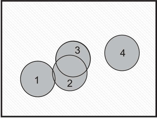
Figure 3: Schematic representation of the way the information provided by different neurons overlap with one another. The stripped area represents the maximum information, namely, $H\{s\}$. Each neuron provides an information $I(1)$, that may fall anywhere in the rectangle. In the case shown here, a significant fraction of the information provided by neurons 2 and 3 is redundant.

For the moment, we assume that the information provided by neuron $N+1$ is either entirely redundant with the one carried by the previous $N$, or the whole of it is new. In other words, neurons provide information in indivisible blocks of size $I(1)$. Later we allow for the possiblility of partial overlap. At the present stage, however, $I$ can only increase in steps of a fixed size, namely of $I(1)$.

With these assumptions, the probability that the information extracted from the response of the neuron $N+1$ is redundant with the information provided by neurons $\left\{1,2,...N\right\}$ is equal to the ratio $I(N)/H\{s\}$. Accordingly, the probability that neuron $N+1$ gives new information is $[H\{s\}-I(N)]/H\{s\}$.

Therefore, the probability that $N+1$ neurons provide an information $I+I(1)$ has two different contributions. On one hand, it may happen that the first $N$ neurons had already provided an information $I+I(1)$, and the information of neuron $N+1$ comes to be redundant to the previous information. Alternatively, it may be that the response of the first $N$ neurons gave an information equal to $I$, and the new neuron provides the extra $I(1)$. We therefore write a recurrence equation for the distribution $f$,

$$f(N+1,I+I(1))=\frac{I+I(1)}{H\{s\}}f(N,I+I(1))+\frac{H\{s\}-I}{H\{s\}}f(N,I).$$ (4)

As a first step, and in order to make the notation simpler, we choose to measure the information in units of $I(1)$. In these units, the maximum information reads $I_{\infty}=H\{s\}/I(1)$. Thus, Eq. (4) reads

$$f(N+1,I+1)=\frac{I+1}{I_{\infty}}f(N,I+1)+\frac{I_{\infty}-I}{I_{\infty}}f(N,I).$$ (5)

This recurrence equation has to be solved with the initial conditions

$$f(0,I) = \delta_{0,I},$$

$$f(N,0) = \delta_{0,N},$$ (6)

where $\delta_{a,b}=1$ if $a=b$, and $\delta_{a,b}=0$ otherwise. The first condition states that no neurons can only give no information, while the second indicates that if there is no information, then, for sure, there are no neurons.

We define a generating function

$$G(x,y)=\sum_{N=0}^{\infty}\sum_{I=0}^{\infty}f(N,I)x^{N}y^{I}.$$ (7)

Clearly,

$$f(N,I)=\frac{1}{N!\ I!}\ \left.\frac{\partial^{N+I}\ G}{\partial^{N}x\ \ \partial^{I}y}\right|_{x=y=0}.$$ (8)

Therefore, if equation (4) is transformed into an equation for $G$, and this last equation is solved, the probability $f$ can be readily calculated, by derivation. Moreover, if we define the mean values

$$\langle I^{j}\rangle=\sum_{I=0}^{\infty}I^{j}f(N,I),$$ (9)

we observe that the first two moments can be obtained with the equalities

$$\left.\frac{\partial G}{\partial y}\right|_{y=1} = \sum_{N=0}^{\infty}\langle I(N)\rangle\ x^{N}$$

$$\left.\frac{\partial^{2}G}{\partial y^{2}}\right|_{y=1} = \sum_{N=0}^{\infty}\left[\langle I^{2}(N)\rangle-\langle I(N)\rangle\right]\ x^{N},$$ (10)

namely, making a series expansion of derivatives of $G$.

It can be shown that the recurrence relation (5) with its initial conditions (6) are equivalent to a differential equation for $G$,

$$\frac{xy}{I_{\infty}}(1-y)\frac{\partial G}{\partial y}+(xy-1)G+1=0,$$ (11)

to be solved with the border conditions

$$G(0,y)=G(x,0)=1.$$ (12)

Morover, since $f$ is a normalized probability distribution,

$$G(x,1)=\sum_{N=0}^{\infty}x^{N}=\frac{1}{1-x}.$$ (13)

The condition $f(N,I>I_{\infty})=0$ implies that $G$ is a polynomial in $y$.

The differential equation (11) for $G$ does not involve derivatives in $x$. Therefore, for each value of $x$ one has an ordinary first order differential equation in $y$, which can be readily integrated. The result is

$$G(x,y) = \frac{y}{1-x}\ _{2}F_{1}\left[1,1-I_{\infty};1+I_{\infty}\frac{1-x}{x};1-y\right]$$ (14)

$$+\frac{I_{\infty}(1-y)}{x+I_{\infty}(1-x)}\ _{2}F_{1}\left[1,1-I_{\infty};2+I_{\infty}\left(\frac{1-x}{x}\right);1-y\right],$$

where ${}_{2}F_{1}$ is Gauss’ Hypergeometric Function (Abramowitz, 1972). It can be easily seen that $G$ fulfills both the border conditions in (12) and the normalization constraint (13). Morover, if $I_{\infty}$ is a positive integer, then the hypergeometric functions in (14) become polynomials in $y$. It may seem, in a first thought, that the requirement of $I_{\infty}$ being an integer is too restrictive. However, if the whole of the striped rectangle in figure 3 is supposed to be filled by blocks of area $I(1)$, it is in fact necessary to have a total area ($H\{s\}$) that is an integer multiple of $I(1)$.

By simple derivation, we get

$$\left.\frac{\partial G}{\partial y}\right|_{y=1}=\frac{x}{(1-x)\left[1-x(I_{\infty}-1)/I_{\infty}\right]}.$$ (15)

This expression involves a linear term in $x$ and two factors that can be written as geometric series. It is therefore easily expanded in powers of $x$. Using equation (10) we obtain

$$\langle I(N)\rangle=\sum_{j=0}^{N-1}\left(\frac{I_{\infty}-1}{I_{\infty}}\right)^{j}=I_{\infty}\left[1-\left(\frac{I_{\infty}-1}{I_{\infty}}\right)^{N}\right].$$ (16)

If instead of writing $I$ in units of $I(1)$ we turn back to bits, equation (16) coincides with (3). In order to state the equivalence of the two, we have to set

$$y=I(1)/H\{s\}=1/I_{\infty},$$ (17)

as was done by Rolls et al(1997).

In figure 4

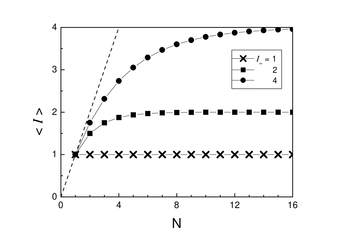
Figure 4: Mean information as a function of the number of neurons sampled, for different values of $I_{\infty}=H\{s\}/I(1)$. The crosses $(\times)$ represent the trivial case of $I_{\infty}=1$. As $I_{\infty}$ grows, the curves rise. In the limit of $I_{\infty}\to\infty$, they approach the dashed line. In all cases, $\langle I(N=0)\rangle=0,\langle I(N=1)\rangle=1$ and $\langle I(N\to\infty)\rangle=I_{\infty}$.

we show $\langle I\rangle$ as a function of $N$, for different values of $I_{\infty}$. The crosses represent the case of $I_{\infty}=1$, where a single neuron provides the maximum information. Obviously, additional cells produce no variation in the mutual information. The squares and the circles represent $I_{\infty}=2$ and $I_{\infty}=4$, respectively. The dashed line shows the behaviour in the limit of $I_{\infty}\to\infty$. All the curves saturate at $I_{\infty}$.

Equation (16) implies that when $I_{\infty}\gg 1$ (or equivalently $I(1)\ll H\{s\}$), the mutual information rises almost linearly with $N$. In fact, expressing $I(N)$ in bits,

$$\lim_{H\{s\}\gg I(1)}I(N)=NI(1).$$ (18)

Therefore, we conclude that for $I(1)\ll H\{s\}$ initially different neurons provide independent information. In the schematic view of figure 3, when the number of neurons is small, they will probably occupy different areas of the striped region. The slope of the initial rise is a measure of the mean information provided by a single unit. The deviation from a strictly linear behaviour is given by the mean pairwise overlap $y=[2I(1)-I(2)]/I(1)$. In all cases, as the number of units is increased, almost the whole of the rectangle is covered, and therefore, the mean information approaches its ceiling. In fact, as $I(1)/H\{s\}$ increases, the initial linear rise is no longer observed, as shown by the squares and in the limit case of the crosses of figure 4.

We now turn to the second moment of the distribution $f$. We define the dispersion

$$\sigma^{2}(N)=\langle I^{2}(N)\rangle-\langle I(N)\rangle^{2}.$$ (19)

Thus, $\sigma$ quantifies how much variability one expects to find in different trials of the random process depicted in figure 3. Or, from the point of view of the experimentalist, the changes that may be expected when $I(N)$ is measured using different sets of $p$ stimuli—keeping them all within the broad class of stimuli to which the cells are supposed do be responsive. Making use of equation (10), we get

$$\sigma^{2}(N) = I_{\infty}\left(I_{\infty}-1\right)\left\{1-2\left(\frac{I_{\infty}-1}{I_{\infty}}\right)^{N}+\left(\frac{I_{\infty}-2}{I_{\infty}}\right)^{N}\right.-$$

$$\left.-\left[1-\left(\frac{I_{\infty}-1}{I_{\infty}}\right)^{N}\right]\left[1-\left(\frac{I_{\infty}-1}{I_{\infty}}\right)^{N-1}\right]\right\},$$

where, for simplicity, $\sigma^{2}$ is written in units of $[I(1)]^{2}$. As expected, $\sigma(N)$ vanishes for $N=0,1,\infty$. In figure

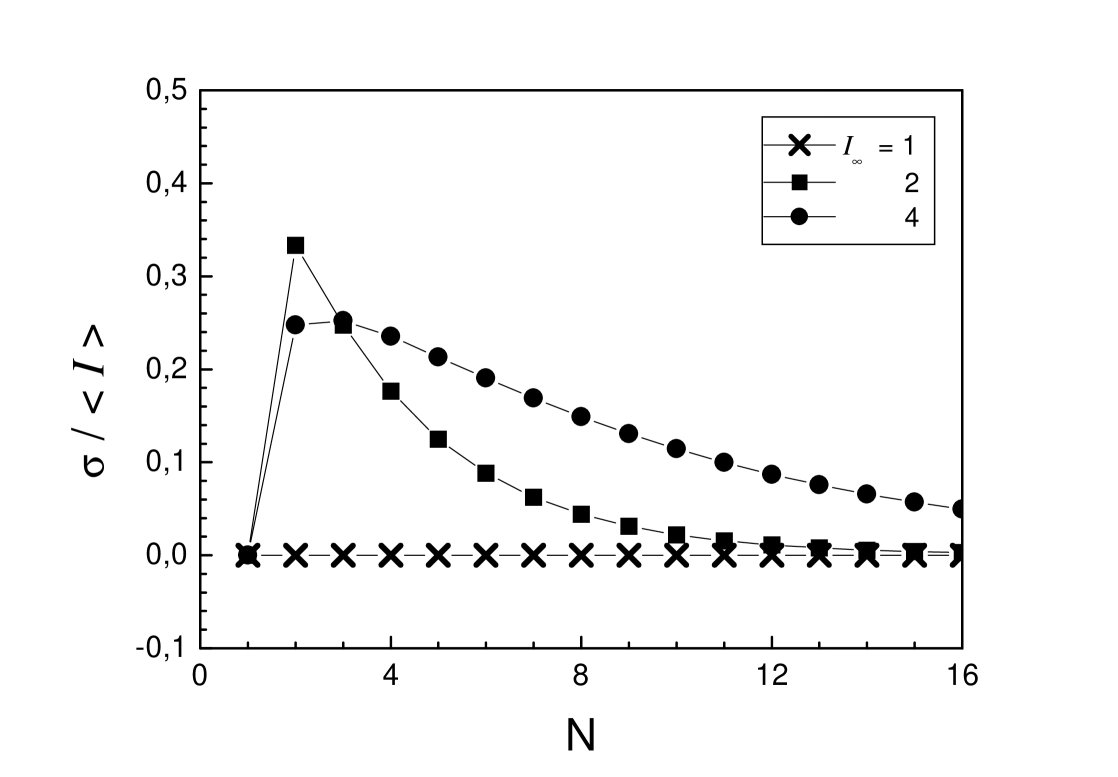
Figure 5: Relative dispersion $\sigma/\langle I\rangle$ (see equation (19))as a function of the number of neurons sampled, for different values of $I_{\infty}=H\{s\}/I(1)$. When $I_{\infty}=1$ and $I_{\infty}\to\infty$, the dispersion vanishes. For intermediate values, we observe a rise in the standard deviation. For all values of $I_{\infty}$ we have that $\sigma(N=0)=\sigma(N=1)=\sigma(N\to\infty)=0$.

5 we plot the relative dispersion $\sigma/\langle I\rangle$ as a function of $N$. We observe that for $I_{\infty}=1$ the standard dispersion vanishes, for all $N$. As $I_{\infty}$ grows, $\sigma/\langle I\rangle$ rises. Its maximum value is reached for $N_{{\rm max}}\approx I_{\infty}$. For very large $I_{\infty}$, the curve flatterns again.

3 Allowing for partial overlaps

Let us now re-formulate the model to allow for the possibility of partial overlap between the information conveyed by any two neurons. Here we present one possible way to do so. Instead of thinking that when one more neuron is considered a whole block of information $I(1)$ is added, we imagine that the same amout $I(1)$ appears in $M$ pieces of size $I(1)/M$. In other words, the information provided by $N$ neurons is the result of sampling at random the whole of the available information a number $N^{\prime}=MN$ of times, each sample of size $I(1)/M$. Ultimately, we shall put $M\to\infty$. We coin $g(N^{\prime},I)$ for the probability distribution that after $N^{\prime}$ steps, an amount $I$ of information is extracted. Clearly, and by analogy with equation (4), $g$ obeys the recurrence relation

$$g(N^{\prime}+1,I+I(1)/M)=\frac{I+I(1)/M}{H\{s\}}g(N^{\prime},I+I(1)/M)+\frac{H\{s\}-I}{H\{s\}}g(N^{\prime},I).$$ (21)

Since we are interested in the information provided by $N$ neurons—and not by $N^{\prime}$ steps—we relate the two probabilities stating

$$f(N,I)=g(MN,I).$$ (22)

This subdivision of the process has two main consequences. First, and as desired, the overlap between the information conveyed by any two neurons in a particular realization is no longer either zero or $I(1)$. Now, the overlap can be any $kI(1)/M$, for integer $k$ varying in $[0,M]$. But in addition, now single neurons do not provide a fixed amount of information. The $M$ blocks of information conveyed by a single neuron may overlap with one another. Therefore, the information provided by just one neuron obeys a distribution ranging from $I(1)/M$ (when all the blocks overlap) up to $I(1)$ (when there is no overlap at all).

In order to solve (21) we choose to measure the information in units of $I(1)/M$. We define

$$I^{\prime} = \frac{I}{I(1)/M}$$

$$I_{\infty}^{\prime} = \frac{H\{s\}}{I(1)/M}.$$ (23)

If the recurrence relation for $g$ is written as a function of $N^{\prime}$ and $I^{\prime}$, equation (5) is obtained, with the only difference that now all variables appear primed. This means that the whole procedure of the previous section can be applied. Using equation (22) to go back to $f$ and taking the limit $M\to\infty$, we get

$$\lim_{M\to\infty}\langle I\rangle=I_{\infty}\left(1-e^{-N/I_{\infty}}\right).$$ (24)

As stated above, in this case, $\langle I(N=1)\rangle$ is not necesarily equal to $I(1)$. Moreover, the whole curve $\langle I(N)\rangle$ differs, in general, from (16). More precisely, the factor $[(I_{\infty}-1)/I_{\infty}]^{N}$ has now been replaced by $\exp(-N/I_{\infty})$. We observe, however, that as $I_{\infty}$ increases, the two results coincide. It can be also shown that in the limit $M\to 0$ the dispersion $\sigma$ vanishes.

The procedure we have devised in order to include the possibility of partial overlaps is equivalent to a re-scaling of the variables $N$ and $I(1)/H\{s\}$. It may be seen that as $M$ grows, the distribution $f(N,I)$ becomes more and more concentrated in its mean value $\langle I(N)\rangle$. In fact, had we attempted to solve equation (4) by taking the continuous limit in the size of the increments of both $N$ and $I$, we would have obtained a solution that is a delta function vanishing for all $I$ and $N$, except for those that obey the equation $I=I_{\infty}[1-\exp(-N/I_{\infty})]$, which is exactly the mean value predicted by (24).

4 Implications for experimental measurements

We have calculated the probability distribution that $N$ neuron provide an amount $I$ of information. We have seen that the mean value of such a distribution is given by equation (3) already proposed by Gawne and Richmond (1993), and further constrained by Rolls et al(1997). The remarkably good accuracy with which equation (3) can fit the real data (see figure 2) suggests that the present approach, although phenomenological, captures the relevant aspects of the way the information about the identity of the stimulus shown is shared among neurons.

The probability distribution characterizes an ensamble of equivalent processes, all of which fulfill two conditions. In the first place, every unit is supposed to provide a fixed amount of information $I(1)$. Rigourously speaking, this assumption is not true, since there is no doubt that some neurons are more informative than others. Our main interest, however, is to derive how the information scales with the number of neurons. We aim at predicting the type of behaviour shown in figure 2. In order to obtain a somewhat universal trend that does not depend on the particular identity and order in which neurons are chosen, it is useful to work with the average single-unit information. Also in the plot of figure 2, each point represents an average over all the possible selections of $N$ neurons ($N$ ranging from one to fourteen), out of the fourteen sampled ones.

Of course, the suposition that every unit provides $I(1)$ bits of information does not mean that there is no trial to trial variability. Whatever the size of the variability—in other words, whatever the distribution $P(r_{j}|s)$—one calculates, using equation (1), the information provided by unit $j$. By averaging this quantity on all $j$, $I(1)$ is obtained.

The second main assumption is that any one neuron provides a random portion of the total available information. When many trials of such a stochastic process are averaged together, one deduces that any two neurons share, on average, a fixed fraction $y$ of $I(1)$. Moreover, when a third neuron is added, the portion of the information that is shared between the three of them is the same fraction $y$ of the mean redundancy between two neurons. In principle, the two fractions need not be the same. In this sense, the present approach is the simplest choice that could be made.

What does this random overlap hipothesis mean, from the point of view of neural operation? If two neurons are strongly correlated (for expample, if they share an appreciable fraction of their imputs) they often provide the same information—more often than by chance. If, on the contrary, the set of neurons is precisely designed so that each unit represents a different feature of the stimuli then, if the stimuli evenly cover the feature space, the information provided by different neurons will seldom overlap—this means, less frequently than by chance. The random overlap hipothesis is, in some way, a null hipothesis. No special organization is assumed, neither in making the neurons particularly redundant nor synergetic. This phenomenological level of description should be contrasted to others approaches, where the correlations among units are described in more detail (Oram et al1998, Abott and Dayan 1999, Panzeri et al1999b, Karbowski 2000). As limited as it might seem, our approach has the appealing property of being analyticaly tractable. Moreover, the resulting $I(N)$ depends on a single parameter $I_{\infty}$.

An alternative to the assumptions made in the present paper would be to model explicitely the conditional probabilities $P({\bf r}|s)$ and calculate $I(N)$ using equation (1), as done in Samengo and Treves (2000). This is a much more detailed level of description, and allows the exploration of different coding strateggies, for example, a localized scheme (sometimes called a grandmother-cell encoding) shows a particular behaviour of $I(N)$, that differs from the one observed in a distributed code. However, such an approach is also much more arbitrary, since a precise model of the unknown parameters shaping the neural responses is needed.

The formalism presented here predicts an average redundancy $y=I(1)/H\{s\}$ entirely determined by ceiling effects. In other words, if the average information provided by each neuron is $I(1)$, then just because the maximum information is finite, there will be a pairwise overlap of $yI(1)$. Therefore, if in an actual experiment the mean redundancy measured is similar to $I(1)/H\{s\}$, this means that there is not much redundancy or synergy in the coding scheme. Such a value stems from the null hypothesis, namely, that neurons share the information at random. It would be therefore interesting to find an experimental overlap that differs signifficantly from $I(1)/H\{s\}$. Or, as suggested by Gawne and Richmond, that the overlaps bear a spatial dependence. That is to say, that even though the overall mean redundancy might be close to $I(1)/H\{s\}$, neurons sitting close to one another could be more redundant than pairs standing further apart.

We would finally like to stress that the saturation of $I(N)$ is only determined by the set of stimuli. One should not deduce that when reaching the ceiling, the pool of neurons has reached its maximum representational capacity. Rather, the stimuli are no longer adequate to explore the coding capabilities of the cells. If an experimentalist is interested in measuring the representational capacity of the system, he or she should choose a set of stimuli whose entropy is large enough so that he can determine precisely the slope of the initial linear rise, that is, $I(1)$. If the aim is to characterize how redundant the messages conveyed by different neurons are, then a measure of the departure from the linear rise is needed. Therefore, $H\{s\}$ should not be extremely large, as compared to $I(1)$. We suggest that a comparison between the measured value of $y$ with $I(1)/H\{s\}$ can indicate if the ceiling effects are only because the set of stimuli is finite, or whether they arise from some special organization in the way different neurons represent information.

References