A Theoretical Search for the Optimum Giant Magnetoresistance

Abstract

The maximum current-perpendicular-to-plane giant magnetoresistance is searched for in magnetic multilayers made of Co, Ni, and Cu with disorder levels similar to those found in room temperature experiments. The calculation is made possible by a highly optimized linear response code, which uses the impurity averaged Green’s function technique and a 9-band per spin tight binding model. Using simulated annealing, hundreds of different configurations of the atomic layers are examined to find a maximum GMR of 450% in ultrathin Ni/Cu superlattices.

The phenomena of the giant magnetoresistance (GMR) has been extensively investigated both theoretically and experimentally since its discovery.Baibich et al. (1988); Binasch et al. (1989) This interest stems from both fundamental questions about magnetism and transport on the nanoscale and also from technological applications like magnetic sensors.Prinz and Hathaway (1995) From this body of work a basic understanding of the physics behind the GMR has emerged. When a magnetic field causes the magnetic domains in a magnetic multilayer or other GMR structure to change their relative orientation, the resistance changes because the bulk and interface scattering rates depend on the electron spin orientation. While this is simple to explain, the actual details are quite complex. Experimentally, it is known that the GMR is very sensitive to atomic composition of the magnetic multilayers. In cases adding a single monolayer can change the magnetoresistance.Parkin (1993) Film growth parameters can similarly change the GMR by an order of magnitude.Colino et al. (1996) The sensitivity to atomic composition and film morphology as well as GMR samples consisting of many atomic layers has made the theory of the GMR challenging (for reviews see Refs. Levy, 1994 and Gijs and Bauer, 1997).

Nonetheless, much progress has been made in elucidating the physics of the GMR in general and in explaining specific experiments. Thus, in this paper we take a different approach. Based on our work and those of other groups, we assume that we have an accurate model of the GMR. Chen et al. (1999) We then ask the question: what is the largest GMR one can obtain for a class of magnetic multilayers with experimentally reasonable disorder parameters? In other words, can one theoretically search the parameter space of a specific class of GMR structures and find the optimum or near optimum atomic configuration? This is a much more challenging problem than computing the GMR for a specific GMR structure because one must perform many individual GMR calculations in the search for the optimum magnetoresistance. Indeed there have been very few calculations like this in condensed matter physics. Franceschetti and Zunger demonstrated the use of simulated annealing to optimize the band gap in semiconductor alloys and superlattices. By searching as much as $10^{4}$ samples, they found the maximum band gap configuration to be very complex.Franceschetti and Zunger (1999) Using a similar approach, Íñiguez and Bellaiche optimized the ground state structural properties and electromachanical response of perovskite alloys.Íñiguez and Bellaiche (2001) This article presents one of the first attempts to optimize a transport property.

Optimizing the transport properties of nanostructures requires a delicate balance between accuracy and speed. To ensure that the optimization results are valid, the model has to include the band structure of the materials, the geometry of the nanostructure, and scattering effects caused by impurities, disorder, and temperature. On the other hand, the calculation of the transport property has to be fast enough that the optimization can be finished in a reasonable amount time. To solve these difficulties, we have developed a highly optimized parallel tight-binding code to compute electron transport in nanostructures using the impurity averaged Green function technique and linear response theory. While the tight binding model we use is not as accurate as other techniques such as density functional theory,Blaas et al. (1999) it does allow us to include realistic band structure efficiently. Similarly, the impurity averaged Green’s function technique allows us to include different kinds of interface and bulk scattering without worrying about the placement of individual defects.

The tight binding Hamiltonian we consider is

$$H=\sum_{{\mathbf{r}},j;{\mathbf{r}^{\prime}},j^{\prime}}H_{{\mathbf{r}},j;{\mathbf{r}^{\prime}},j^{\prime}}c^{\dagger}_{{\mathbf{r}},j}c_{{\mathbf{r}}^{\prime},j},$$ (1)

where ${\mathbf{r}}$ and ${\mathbf{r}}^{\prime}$ are sites on the lattice. The indices $j$ and $j^{\prime}$ denote one of the one s, three $p$, or five d levels and also the spin orientation. Within a tight binding model, the disorder comes from variations in the matrix elements. In the impurity averaged green function technique, these variations are treated statistically by averaging over an ensemble of different microscopic configurations of the disorder with the same macroscopic properties, e.g., density of impurities. Denoting this average by angular brackets, our unperturbed Hamiltonian is $H_{o}=\langle H\rangle$. The deviation from this average for a particular configuration of the disorder is given by $\delta H=H-H_{o}$.

Scattering is included through the choice of the self-energy. We use the self-consistent Born approximation with uncorrelated disorder fluctuations. For energy $\omega$ the retarded and advanced self-energies, $\Sigma^{\textrm{R}/A}$, are expressed in terms of the retarded and advanced green functions, $G^{\textrm{R}/A}$ as

$$\Sigma^{\textrm{R}/A}_{{\mathbf{r}},j;{\mathbf{r}},j}(\omega)=\langle(\delta H_{{\mathbf{r}},j;{\mathbf{r}},j})^{2}\rangle G^{\textrm{R}/A}_{{\mathbf{r}},j;{\mathbf{r}},j}(\omega),$$ (2)

where the green function is in turn expressed in terms of the self-energy via

$$[\omega-H_{o}-\Sigma^{\textrm{R}/A}(\omega)]G^{\textrm{R}/A}(\omega)={\mathbf{1}}.$$ (3)

This last equation is a matrix equation, where the ${\mathbf{r}}$ and $j$ indices have been suppressed.

Within the linear response theory, the conductivity is computed via the Kubo formula. For the geometry with the current flowing perpendicular to the planes (CPP) it is necessary to include the vertex correction, $\Gamma$, which is given by the self-consistent equation,

$${\mathbf{\Gamma}}_{{\mathbf{r}},j;{\mathbf{r}},j}=\langle(\delta H_{{\mathbf{r}},j;{\mathbf{r}},j})^{2}\rangle\left(G^{\textrm{R}}({\mathbf{J}}+{\mathbf{\Gamma}})G^{\textrm{A}}\right)\Big{|}_{{\mathbf{r}},j;{\mathbf{r}},j},$$ (4)

where ${\mathbf{J}}$ is the current operator,

$${\mathbf{J}}_{{\mathbf{r}},j;{\mathbf{r}^{\prime}},j^{\prime}}=-i({\mathbf{r}}-{\mathbf{r}^{\prime}})H_{{\mathbf{r}},j;{\mathbf{r}^{\prime}},j^{\prime}}.$$ (5)

A conserving approximation for the conductivity at ${\mathbf{r}}$ is

$$\sigma_{\alpha\beta}(\mathbf{r}) = \frac{e^{2}}{h}\mbox{Tr}\{J_{\alpha}({\mathbf{r}})G^{\textrm{R}}(J_{\beta}+\Gamma_{\beta})G^{\textrm{A}}$$

$$- \frac{1}{2}J_{\alpha}({\mathbf{r}})G^{\textrm{R}}J_{\beta}G^{\textrm{R}}-\frac{1}{2}J_{\alpha}({\mathbf{r}})G^{\textrm{A}}J_{\beta}G^{\textrm{A}}\},$$

where ${\mathbf{J}}({\mathbf{r}})$ is the local current density operator at ${\mathbf{r}}$. The sum of ${\mathbf{J}}({\mathbf{r}})$ over position times the lattice unit cell volume is equal to the current operator in Eq. (5). In the CPP geometry this conductivity will be constant because the current density is independent of position.

Letting $\sigma_{\textrm{F}}$ be the conductivity when the magnetic layers are aligned ferromagnetically and $\sigma_{\textrm{A}F}$ be the conductivity when adjacent magnetic layers are aligned antiferromagnetically, the giant magnetoresistance is defined as ${\textrm{G}MR}=(\sigma_{\textrm{F}}-\sigma_{\textrm{A}F})/\sigma_{\textrm{A}F}$. Note that in practice the magnetic layers will not necessarily be aligned antiferromagnetically at zero field; however, our simulation does not compute the magnetic domain structure, but only the conductivity. In particular some of the ultrathin magnetic layers which we find with large GMR could very well be ferromagnetically coupled.Parkin et al. (1990) It is possible to achieve antiparallel alignment even with ferromagnetic coupling by going to a spin valve geometry with only two magnetic layers where one of the layers is exchange biased.Dieny et al. (1991)

An optimization study involves many GMR calculations, therefore, the speed for each GMR calculation is crucial. The trace in Eq. (6) is over all positions and atomic levels; however, since the system is periodic, it can be broken up into a sum in k-space and a sum within a unit cell. Thus, the matrices are of order $9N$ for each spin, where $N$ is the number of atoms in a unit cell. At first glance, the matrix products and inverses in Eqs. (3), (4) and (6) are all $O(N^{3})$ operations, where $N$ is the number of atoms in the unit cell. In addition, both Eqs. (3) and (4) are self-consistent equations. Performing optimization with a self-consistent $O(N^{3})$ implementation is estimated to take about 5 CPU-years, which is impractical. To overcome this, we have developed an $O(N)$ algorithm to solve Eqs. (3) and (6), and an $O(N^{2})$ algorithm to solve Eq. (4) directly without the need for iteration. For $N=50$, this algorithm is more than 100 times faster than the $O(N^{3})$ algorithm. Running on a Linux cluster of five dual 866MHz Pentium III CPU workstations, it takes about 20 minutes for each GMR calculation and about two weeks for an optimization.

The optimization technique we use is simulated annealing. Since not every configuration qualifies as a GMR structure, the optimization is performed in the constrained subspace consisting of a unit cell with two magnetic layers separated by two non-magnetic spacer layers. After an arbitrarily chosen initial unit cell, each subsequent configuration is generated by one of the following Monte Carlo moves: (i) inserting a monolayer, (ii) removing a monolayer, or (iii) changing the composition of a monolayer. If the GMR of the new configuration is higher than the previous configuration, then it is accepted. On the other hand, if the new GMR is lower, it is only accepted with a probability of $\exp(\Delta\mbox{GMR}/T)$, where $\Delta\mbox{GMR}$ is the change in the GMR and $T$ is the simulated annealing temperature. The process is continued as the annealing temperature is gradually lowered until there is no further change in the configuration and a final near-global maximum in the GMR is attained.

In the following, we show results of a study that looks for the optimal configuration of superlattices made with Co, Ni, and Cu in conditions similar to GMR experiments at room temperature. To make the study more manageable, we only consider fcc (111) lattices. The minimum thickness of each layer is limited to two monolayers in order to avoid complications such as pin holes. The tight binding parameters in Eq. (1) are obtained from fits to density-functional calculations where up to second-nearest-neighbor hoping energies are included.

Two types of scattering are included: spin-independent scattering and spin-dependent scattering. The spin-independent scattering represents the structural disorder and is included in the calculation by uniformly shifting all the orbital levels at a site: $\langle(\delta H_{{\mathbf{r}},j;{\mathbf{r}},j})^{2}\rangle=0.2{\textrm{e}V}^{2}$, which corresponds to a Cu resistivity of 3.1 $\mu\Omega{\textrm{c}m}$, about twice the value of clean Cu at room temperature. The spin-dependent scattering is assumed to be due to inter-diffusion of atoms near the interface. It is modeled by the shifting of the d-levels only, since the d-levels are the primary difference in the tight binding parameters for these elements. The shift in the d-levels are determined by fits to 4-atom supercell density-functional calculations of an impurity in three host atoms. We then assume an interface mixing percentage of 10% in each of the two monolayers on either side of the interface. The value of $\langle(\delta H_{{\mathbf{r}},j;{\mathbf{r}},j})^{2}\rangle$ for the majority and minority d-states is equal to 0.29 and 0.84 ${\textrm{e}V}^{2}$ at the Co/Cu interface, and 0.03 and 0.11 ${\textrm{e}V}^{2}$ at the Ni/Cu interface. Using these parameters, the GMR for a [Co₃/Cu₃/Co₃/Cu₃] superlattice is 36%, which is in the range of observed CPP-GMR at room temperature.Gijs et al. (1994) Our spin-dependent scattering does not include spin flip scattering, which can be important for short spin flip scattering lengths.Valet and Fert (1993)

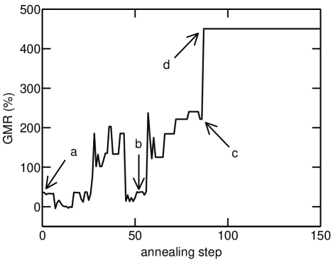
Figure 1: GMR as a function of the simulated annealing step. The four marked configurations and their GMR values are: (a) [Co₃/Cu₃/Co₃/Cu₃] $36\%$, (b) [Ni₂/Cu₃/Ni₂/Cu₂] $221\%$, (c) [Ni₂/Cu₂/Ni₂/Co₁/Cu₂] $38\%$, and (d) [Ni₂/Cu₂/Ni₂/Cu₂] $450\%$. Notice that the GMR is very sensitive to the configuration. Both (b) and (c) differ from (d) by only one monolayer.

The giant magnetoresistance for a simulated annealing run is shown in Fig. 1. The initial configuration has been chosen to be the superlattice [Co₃/Cu₃/Co₃/Cu₃], with a unit cell made of four layers, each consisting of three monolayers of either Co or Cu. The particular choice of initial configuration does not effect the final result for this calculation. As the annealing temperature $T$ decreases from its initial value of $60\%$, the GMR becomes larger. The GMR does not increase monotonically because a superlattice that reduces the GMR is accepted with a probability set by the Boltzmann factor, which is crucial for escaping from local maxima in the GMR. As the annealing temperature is lowered, the chance of leaving a local maximum becomes smaller and smaller. At step 89 in this run, the GMR jumps to $450\%$ and no other configurations are accepted. The atomic configuration for the highest GMR (d) is [Ni₂/Cu₂/Ni₂/Cu₂]. This is a very surprising result because most room temperature studies to date have GMR values less than $100\%$.Gijs et al. (1994); Gijs and Bauer (1997); Bass and Pratt (1999) From Fig. 1 one can see that the GMR is very sensitive to the atomic configuration. For example, superlattices (b) and (c) have GMR values of 221% and 38%, respectively, yet they differ by only one monolayer from the optimal GMR of superlattice (d), 450%.

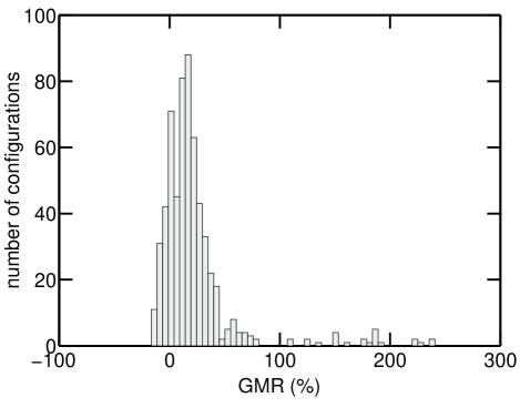
Figure 2: Histogram of the GMR in the configuration space for 600 randomly generated configurations. The average GMR is $22\%$, and the standard deviation is $36\%$. About $97\%$ of the configurations are located near the main peak with GMR values less than 100%, while 3% of the configurations are many standard deviations away from the main peak with GMR values greater than 100%. These large GMR configurations are mostly ultrathin Ni/Cu superlattices.

To get a better picture of the GMR in configuration space, we have calculated the GMR for 600 randomly generated configurations. The result is shown in Fig. 2 as a histogram. The average GMR is $22\%$, and the standard deviation is $36\%$. There are two groups of configurations. About $97\%$ of the configurations are located near the main peak. They have a GMR less than $100\%$. On the other hand, about $3\%$ of the configurations have GMR many standard deviations away from the main peak. They scatter in the range from $100\%$ to $450\%$. Most of the large GMR configurations are ultrathin Ni/Cu superlattices. Only two of the large GMR configurations contain Co. Since the large GMR configurations are rare, they may have been overlooked.

What causes the GMR to be large in some multilayers but not others? The dominant source of scattering in these transition metals is due to s-d hybridization. The d-levels in the majority spin of Ni, Co, and Cu are below the Fermi level; however, there is still a finite d-density of states at the Fermi level due to both s-d hybridization and disorder. In particular disorder can substantially smear the d-density of states, increasing the value at the Fermi level.Chen et al. (1999) Since the d-levels in Ni and Cu are more well matched than those in Co and Cu, the disorder due to interface mixing is smaller in Ni/Cu multilayer than in a Co/Cu multilayer. Thus, the GMR is greater in a Ni/Cu multilayer for the same level of interface mixing because scattering via the s-d hybridization is less.

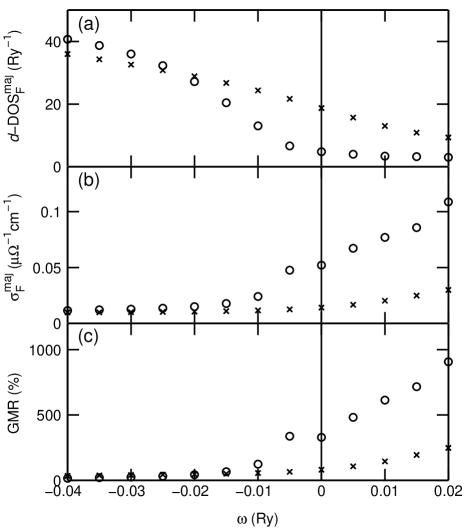
Figure 3: Comparison of [Ni₂/Cu₂/Ni₂/Cu₂] (circles) and [Co₂/Cu₂/Co₂/Cu₂] (crosses) superlattices. (a) At the Fermi level the d-density of states for the majority spin when the magnetic layer aligns ferromagnetically, d-DOS${}_{\textrm{F}}^{\textrm{m}aj}$, is higher in the Co/Cu sample, leading to higher scattering. (b) The conductivity for the same spin channel, $\sigma_{\textrm{F}}^{\textrm{m}aj}$, in Co/Cu is thus lower than that in Ni/Cu. Since near the Fermi energy the conductivities for the minority spin and the antiferromagnetically aligned magnetic layers are relatively small and flat compared with $\sigma_{\textrm{F}}^{\textrm{m}aj}$, the GMR (c) resembles $\sigma_{\textrm{F}}^{\textrm{m}aj}$.

To see this more clearly, in Fig. 3 we take a representative Ni/Cu sample and a representative Co/Cu sample. The two samples have the same bulk disorder, but the Ni based multilayer actually has more interface mixing (10%) than the one containing Co (5%) to allow the curves to fit clearly on the same plots. As seen in Fig. 3(a), the d-density of states is smaller in the Ni sample. The d-density of states correlates well with the larger conductivity shown in Fig. 3(b) and the larger GMR shown in Fig. 3(c). The fact that there is a simple explanation for this large GMR indicates that it is a robust effect and not strongly dependent on the many assumptions which we have made. Also, it says that for comparable coupling between layers and disorder, the Ni/Cu multilayers will have a larger GMR than the Co/Cu ones.

In this paper we have performed a simulated annealing search for the optimum or maximum giant magnetoresistance by varying the atomic composition of multilayers composed of Ni, Co, and Cu. The disorder parameters in our calculation were chosen to simulate room temperature experimental conditions. After hundreds of GMR calculations for different atomic configurations, a surprisingly large GMR was found for ultrathin Ni/Cu multilayers. The origin of this large GMR of 450% was found to be the fact that the d-levels in Ni and Cu are relatively close in energy. Thus, although we have made a number of approximations in order to perform our calculation in a reasonable amount of time, the large GMR appears to be a robust effect. We believe that this work is part of a large class of problems in tailoring transport properties of nanostructures to optimize an observable such as the magnetoresistance.