Mechanistic approach to generalized technical analysis of share prices and stock market indices

Abstract

Classical technical analysis methods of stock evolution are recalled, i.e. the notion of moving averages and momentum indicators. The moving averages lead to define death and gold crosses, resistance and support lines. Momentum indicators lead the price trend, thus give signals before the price trend turns over. The classical technical analysis investment strategy is thereby sketched. Next, we present a generalization of these tricks drawing on physical principles, i.e. taking into account not only the price of a stock but also the volume of transactions. The latter becomes a time dependent generalized mass. The notion of pressure, acceleration and force are deduced. A generalized (kinetic) energy is easily defined. It is understood that the momentum indicators take into account the sign of the fluctuations, while the energy is geared toward the absolute value of the fluctuations. They have different patterns which are checked by searching for the crossing points of their respective moving averages. The case of IBM evolution over 1990-2000 is used for illustrations.

Keywords: Econophysics; Force; Momentum; Energy; Pressure; Acceleration; Mass; Volume; Price; Technical Analysis; Market Indices; Stocks

I Introduction

Technical indicators as moving average and $momentum$ are part of the classical technical analysis and are much used in efforts to predict market movements.[1, 2, 3] One question is whether these techniques provide adequate ways to read the trends, and later on allow for an investment strategy development. It has been shown that moving average trading rules can be utilized [4, 5] for USA and UK markets. In both futures and spot foreign currency markets significant profits can be earned along these lines.[6] Parisi and Vasquez recently used the moving average technique on emerging markets [7] to show that buy signals consistently generate higher returns than sell signals. Moreover, returns following sell signals are shown to be negative, which is not easily explained by any of the currently existing equilibrium models. Related studies by Gunasekarage and Power [8] also showed that technical trading rules have predictive ability in South Asian stock markets.

One surprise to a physicist is the neglect of the volume of transactions in the classical way of predicting the evolution of a share price or a market index. Yet there was a sort of thermodynamic relationship between share price and exchanged volume of shares in estimating the value of some company from an investor point of view.[9, 10] Such an addition to measure and if possible predict the evolution of stocks is introduced here. Indeed we present a generalization of the classical technical analysis concepts taking into account the volume of transactions. The latter becomes a time dependent or generalized mass. The notions of pressure, acceleration and force are deduced. In that spirit, a generalized (kinetic) energy is easily defined. It is pointed out that the momentum correlations take into account the sign of the fluctuations, while the energy is geared toward the absolute value of the fluctuations. They have different patterns which are checked by searching for the crossing points of their respective moving averages. The evolution of IBM share price and volume between Jan 01, 1990 and Dec 31, 2000 is used for illustrations.

II Technical Analysis

A Moving Average

Consider a time series $x(t)$ given at N discrete times $t$. The series (or signal) moving average $M_{\tau}(t)$ over a time interval $\tau$ is defined as

$$M_{\tau}(t)=\frac{1}{\tau}\sum_{i=t}^{t+\tau-1}x(i-\tau)\qquad t=\tau+1,\dots,N$$ (1)

i.e. the average of $x$ over the last $\tau$ data points. For simplicity we suppose that the ticking times are equally spaced. One can easily show that if the signal $x(t)$ increases (decreases) with time, $M_{\tau}(t)<x(t)$ ($M_{\tau}(t)>x(t)$). Thus, a moving average captures the past trend of the signal over a given time interval $\tau$. The IBM daily closing value price signal between Jan 01, 1990 and Dec 31, 2000 is shown in Fig. 1 (top figure) together with the $\tau=50$ day moving average taken from Yahoo.[11] The bottom figure shows the daily $volume$ of transactions given in millions.

The moving average notion has already been discussed.[12, 13] It is obvious that like any other statistical $mean$, a moving average $M_{\tau}(t)$, depends on the number of data points taken into account. There can be as many moving averages as $\tau$ intervals. The shorter the $\tau$ interval the closer to a signal is the moving average. However, a too short moving average may give false messages about the long time trend of the signal. In Fig. 2 two moving averages of the IBM signal for $\tau$=5 days (i.e. 1 week) and 21 days (i.e. 1 month) are compared for illustration.

The intersections of the $price$ signal with a moving average can define so-called lines of $support$ or $resistance$.[1] A support (resistance) line occurs when the local minimum (maximum) of $x(t)$ bounces on $M_{\tau}(t)$. The lines are supposed to indicate the price level at which $\tau$-investors believe that prices will move higher or lower respectively. In Fig. 2, IBM lines of resistance happen e.g. around June 1993 and lines of support around mid Oct. 1993 for the $\tau$ = 5 days and 21 days cases respectively. Support and resistance levels depend on $\tau$ and are based in principle on investment horizon strategy, but are in fact containing much psychological fancy.

Other features of the moving average prone investor framework are the intersections between $two$ moving averages $M_{\tau_{1}}$ and $M_{\tau_{2}}$. They might occur or not at drastic changes in the trends of $x(t)$.[12] Consider again the two moving averages of IBM price signal for $\tau_{1}=5$ days and $\tau_{2}=21$ days (Fig. 2). If $x(t)$ increases for a long period of time before decreasing rapidly, $M_{\tau_{1}}$ will cross $M_{\tau_{2}}$ from above. This event is called a death cross in empirical finance.[1] In contrast, when $M_{\tau_{1}}$ crosses $M_{\tau_{2}}$ from below, the crossing point is a gold cross. They appear more drastic when the respective slopes have different signs. In Fig.2 a death cross and a gold cross occur near March 93 and Oct. 93 respectively. The density of such crossing points between two moving averages as a function of the difference in the characteristic $\tau$’s defining the moving averages has been discussed elsewhere[12] and is shown in Fig.3 for the case of interest here. Based on this idea, a new and efficient approach has been suggested in order to estimate an exponent that characterizes the roughness of a signal. From Fig.3 and Ref.[12] the IBM roughness exponent has been found equal to $0.44\pm 0.02$ for the time interval considered.

B Momentum Indicator

The so called momentum[1] is another instrument of the technical analysts. We will refer to it here as the classical momentum for reasons to become obvious later. The classical momentum of a stock is defined over a time interval $\tau$ as

$$R_{\tau}(t)=\frac{x(t)-x(t-\tau)}{\tau}=\frac{\Delta x}{\Delta t}\qquad t=\tau+1,\dots,N$$ (2)

For $\Delta t$ =$\tau$ = 1, the momentum is nothing else than the volatility. The momentum $R_{\tau}$ for three time intervals, $\tau$=5, 21 and 250 days, i.e. one week, one month and one year, are shown in Fig. 4 for IBM between 1990 and 2000, together with a blow up for the years 1999-2000. The longer the period, the smoother the momentum signal. Relevant information on the price trend turnovers is usually considered to be found in a few moving averages of the $momentum$, or momentum indicator, i.e. in

$$R^{\Sigma}_{\tau}(t)=\sum_{i=t}^{t+\tau-1}\frac{x(i)-x(i-\tau)}{\tau}\qquad t=\tau+1,\dots,N$$ (3)

like those for $\tau$ = 1 week, 1 month and 1 year. Notice that those are calculated over the same time intervals over which the momentum is calculated. For IBM, these $R^{\Sigma}_{\tau}$ are shown in Fig. 5. The density of intersections between moving averages of these momenta could be calculated. The result is displayed in Fig.3.

C Classical Strategy

In Fig. 6 the IBM signal and its weekly (short-term), monthly (medium-term) and yearly (long-term) moving averages are compared to the weekly (short-term), monthly (medium-term) and yearly (long-term) momentum indicators to show the 1999 bullish and also beginning of bearish trends. The strategic message that is coming out of reading the combination of these six indicators (Fig. 6) is that one could start buying at some momentum bottom and sell at a maximum. A buy position is found for both monthly and weekly momentum indicators around (1) Feb. 99. Another buy position occurs around mid-April 99 when the price surge confirms the momentum uptrend, at a gold cross (2). Selling signals are given at the maximum of the monthly momentum indicator in mid-Jan. 99 (6), near the second half of mid-May (7) and mid-July (8). A death cross (3) occurs between the short and medium term moving averages in Sept. 99 and is subsequently followed by the maximum (4) of the monthly momentum, even turning negative. In Oct. 99, occurs the maximum of the long-term momentum, just before the Oct. 99 crash (5). A good technical analyst would have strongly recommended to sell the position since the price is also falling down below the weekly moving average. Hope (or faith?) for prospect reoccurs after Nov. 99 during one month.

III Generalized technical analysis

Stock markets do have another component beside prices or volatilities. This is the volume of transactions. It is introduced here as the physical mass of stocks. Remember that the number of shares is constant over rather long time intervals, i.e. usually between splits, like the mass of an object.

Consider $V(t)$ to be the volume of transactions of a stock with price $x(t)$ at time $t$, - Fig. 1 (bottom). A generalized momentum $\widetilde{R}_{\tau}$ over a time interval $\tau$ can be defined (see Fig. 7) as in physics through

$$\widetilde{R}_{\tau}(t)=\frac{V(t)}{<V(t)>_{\tau}\tau}\cdot\frac{x(t)-x(t-\tau)}{\tau}=m(t)\frac{\Delta x}{\Delta t},\qquad t=\tau+1,\dots,N$$ (4)

where the total volume of transactions over the interval $\tau$ is $<V>_{\tau}\tau=\sum_{i=1}^{\tau}V(i)$. In so doing, we introduce some financial analogy to a generalized time dependent mass $m(t)$ of a diffusing object. The total volume in the denominator is introduced for a normalization purpose. Notice that we could choose other normalizations or definitions of the mass or the generalized momentum : one could take the $log(V(t))$, but this introduces a nonlinear transformation. One could use $log[V(t+\tau)/V(t)]$ but that can be negative. One could normalize with respect to $<V>_{\tau}$ only, but $\widetilde{R}_{\tau}(t)$ values would be larger, ….

In order to search for more definite indications on the stock trend changes, represented as the complex influence between price and volume of transactions, we further consider a moving average of the generalized momentum, i.e. a generalized momentum indicator (Fig.8) which is

$$\widetilde{R}^{\Sigma}_{\tau}(t)=\sum_{i=t}^{t+\tau-1}\frac{V(t)}{<V>_{\tau}\tau}\cdot\frac{x(i)-x(i-\tau)}{\tau}\qquad t=\tau+1,\dots,N$$ (5)

The IBM generalized momentum indicator $\widetilde{R}_{\tau}$ for three time intervals $\tau$, i.e. 1 week, 1 month and 1 year and their corresponding moving average $\widetilde{R}^{\Sigma}_{\tau}$ are shown in Fig. 8. It is observed that the multiplicative factor results only in enhancing features, i.e. the mass being here positive. However the slopes in the generalized momentum indicator are much enhanced due to volume variations. A comparison of moving averages of the IBM signal and its IBM generalized momentum for three different horizons together with the volume of transactions are shown in Fig. 9. The volume of transactions is plotted in tenths of millions on the generalized momentum base line. The long-term (yearly) generalized momentum signal is marked by dot-dash curve and has small positive values, with a steady increase up to the maximum of the IBM price around mid Sept. 1999 marked by the index (3). See the well marked crash of Oct. 99; also displayed in Fig.9, just after (5). The crash coincides with the maximum in the volume of transactions, and a negative momentum.

A closer look of the short (weekly) and medium-term (monthly) momentum in terms of sell/buy message point of views again suggests to buy around Feb. 1999 (see Fig. 6 as well) at the minimum of the momentum curve. The new feature is that the peaks of the generalized medium term (monthly) and long-term (yearly) momentum enhances several changes in the price trend represented by its monthly or yearly moving average. Peaks are observed at mid Jan. 99 (6), mid May (7) (after the gold cross (2) ) and mid July 1999 (8). Notice that (3) and (8) coincide with the monthly momentum turning to negative values after reaching a weak maximum. Notice the differences between Fig. 6 and Fig. 9, i.e. the enhanced, and even modified structures, between (6) and (1), and between (4) and the Oct. crash, due to the volume effect.

A Pressure, Acceleration and Force Indicators

Introducing a ”mass” $m(t)=V(t)/(<V>_{\tau}\tau)$ and the ”velocity” $v(t)=\Delta x/\tau$ through the standard notion of physical momentum

$$\widetilde{R}^{\Sigma}_{\tau}=p(t)=\sum_{i=t}^{t+\tau-1}m(i)v(i)$$ (6)

enables us to take into account both sides of the market coin and their impact on one another.

Note that $<V>_{\tau}\tau$ ensures to include a $pressure$ contribution from the variation of the accumulated volume of transactions during the time period $\tau$ on the change of the momentum of the stock. From a mathematical point of view at the time of the peaks of generalized momentum curve $\widetilde{R}^{\Sigma}_{\tau}$, the first derivative of the momentum are obviously equal to zero and the second derivative is negative or positive depending whether there is a peak or a dip. Because of the time dependent ”mass” this implies that

$$p^{\prime}(t)=\sum_{i=t}^{t+\tau-1}m^{\prime}(i)v(i)+\sum_{i=t}^{t+\tau-1}m(i)v^{\prime}(i)=0$$ (7)

or

$$p^{\prime}(t)=\sum_{i=t}^{t+\tau-1}m^{\prime}(i)v(i)+\sum_{i=t}^{t+\tau-1}m(i)a(i)=0,$$ (8)

where $a(i)$ can be thought as an $acceleration$. Therefore the second term in Eq. 8 represents a classical $force$ that acts upon the object (stock or market index). It originates from the speed of change of stock price whose sign is either positive or negative. At times of extrema this force balances the first term in Eq. 8, determining the rate in the volume of transactions. The sign of this first term depends on the accumulated sum of $m^{\prime}(i)v(i)$, since both $m^{\prime}(i)$ and $v(i)$ can be negative or positive.

Therefore, the fact that the first derivative of the momentum $p^{\prime}(t)$ vanishes at time $t_{1}$ can lead to a deeper reading of the price/volume interactions. The maximum of the (generalized or not) momentum indicator at $t_{1}$, mid Jan. 1999, mark (6) in Fig. 6 and Fig.9, is related to a sharp increase of the volume of transactions, as the rescaled volume of transactions is of the order of $\widetilde{R}^{\Sigma}_{\tau}$. For Eq. 8 to be satisfied, the second term in the equation should be negative. Thus the derivative of the $velocity$, i.e. the acceleration $\Delta v(t)/\Delta t$ should be negative, which means a change in the derivative of the price trend. This is easily seen at the resistance point, that also coincides with a death cross between the IBM signal and its moving averages for the one week and one month time averaging at (1). The same discussion pertains to the maximum of the momentum curve in mid July 1999, mark (8) in Fig. 6 and Fig. 9, when the IBM share price breaks the resistance line, just before a death cross when the price drops below its monthly moving average, while the weekly moving average becomes negative.

However, the cause of the peak in the generalized momentum indicator at mid-May, 1999, mark (7) in Fig. 6 and Fig. 9, is more complex than for mid-Jan. 99, mark (6), or mid-July 99, mark (8). Indeed the acceleration during most of the two prior months is positive and so is the second term in Eq. 8. At the time of the price maximum on May 13, 1999 the classical force has to be (and is) balanced by a (negative) contribution from the first term. Because the velocity $v(i)$ is positive during that period, the derivative of the volume of transactions (the mass) has to be (and is) most of the time negative.

Thus the increase of momentum is not entirely due to the price increase, but does have another component, hidden if one does not consider the above generalization. After May 13, 1999, the price drops to the monthly moving average and rebounds on a support line. Thus this can be interpreted as a continuous price increase with corrections to the moving average price due to the influence of the volume of transactions. The observed evolution of the generalized momentum of the IBM stock implies that some generalized force can be considered as a cause of these changes.

B Energy

Mechanically speaking it can be thought that some $energy$ is also accumulated through the interplay between the price and the volume of transactions and causes a generalized force to act. Therefore, a kinetic ”energy” can be introduced as

$$E^{\Sigma}_{\tau}(t)=\sum_{i=t}^{t+\tau-1}\left(\frac{x(i)-x(i-\tau)}{\tau}\right)^{2}\qquad t=\tau+1,\dots,N.$$ (9)

The generalized mass introduced above leads also to generalize the ”energy” of the stock signal to be like in mechanics (we drop the factor $1/2$)

$$\widetilde{E}^{\Sigma}_{\tau}(t)=\frac{1}{\tau}\sum_{i=t}^{t+\tau-1}\frac{V(t)}{<V>_{\tau}}\cdot\left(\frac{x(i)-x(i-\tau)}{\tau}\right)^{2}\qquad t=\tau+1,\dots,N$$ (10)

or

$$\widetilde{E}^{\Sigma}_{\tau}(t)=m(t)\left(\frac{\Delta x}{\Delta t}\right)^{2}=mv^{2}.$$ (11)

Theoretical and generalized $energy$ of the IBM stock are shown in Figs. 10-11 for the same three usual time interval averages $\tau$, i.e. one week, one month, one year. Note (insert of Fig. 10) two large peaks in the monthly theoretical energy : the high one in mid-May 1999 corresponding to (7) in Fig. 9, and one at the crash time in October. A small peak in mid-July, mark (8) in Fig. 9, corresponds to the maximum of the price and the generalized momentum. The appearance of a huge increase in energy in Oct. 99 together with the negative slope of the generalized momentum indicator should be interpreted now as a serious warning for an incoming crash. A mimimum in kinetic energy can be seen to provide information on strong continuing price increase or decrease depending on the momentum rate of change. The local maximum of a kinetic energy as in classical physics indicates some accumulation of energy at that time for the evolution of the stock, - accumulation which must be dissipated ! It is interesting to note that the monthly generalized energy (Fig. 11, inset) emphasizes even further the huge accumulation of energy in Oct. 1999.

IV Conclusions

A thermodynamic-like phase diagram between the daily closing price ($P$) and the daily transaction volume ($V$) resulted in a fundamental phase diagram for companies quoted on stock exchanges.[9] This pointed out to search for correlations between volume and price. In the same spirit of econophysics connecting physics and financial data for share prices or stock market indices we have developed a generalization of the classical method by technical analysts, i.e starting from the notion of moving averages and momentum indicators.[1] One can take into account not only the price of a stock but also the volume of transactions which is similar to a time dependent generalized mass in mechanics. This might interestingly serve for generalizing ideas on anomalous diffusion model(s)[16] for price evolutions as well. A notion of pressure, acceleration and force concepts are deduced and identified to their classical mechanics counterparts. The terms have sometimes been used in the literature but outside their classical meaning.[17] A generalized (kinetic) energy is also easily defined, in the same lines of an analogy. A correspondence between mechanical terms, classical technical analysis terms and to be seen generalized concepts of technical analysis is found in Table I. This might help in devising a free energy like approach, as also introduced elsewhere.[18]

Introducing the product of price and mass of transactions in indicators renders the new signals very rough. The number of intersections, mimima and maxima is highly modified. Whether the above generalization of technical analysis concepts can be used to increase the number of buy/sell orders, and develop new strategies through nine rather than six indicators (shown as a summary in Figs. 12-13) is left for further work. The interest of such considerations will be obvious if cumulated (good !) predictions[19] from the above stand over usual findings.

Finally it seems that the (generalized) momentum and energy concepts so introduced concern other effects studied in economy, i.e. the correlation existence of signs and amplitudes of share price variations. It is easily understood that the momentum (and momentum correlations) take into account the sign of the fluctuations (and their correlations), while the energy (and energy correlations) is geared toward the absolute value of the fluctuations (and their correlations). In thermodynamics of non-equilibrium processes, these correlations are described by the $viscosity$ and thermal conductivity coefficient respectively. Thus the above concepts might also serve in a dynamic equation framework.

Acknowledgements

MA thanks Etienne Labie and Denis Vanderborght (Leleux Ass.) for practical comments and references.

classical			classical		generalized
mechanics			technical analysis		technical analysis
mass	$m(t)$	$V(t)$	(Volume)	$V(t)$	Volume
distance	$x(t)$	$x(t)$	price	$x(t)$	price
trend	$<x(t)>$	$<x(t)>$	moving average	$<x(t)>$	moving average
momentum	$m(t)v(t)$	$\Delta x(t)/\Delta t$	momentum	$V(t)x^{\prime}(t)$	generalized
					momentum
kinetic	$m(t)v^{2}(t)$	$<(\Delta x(t)/\Delta t)^{2}>$	(kinetic	$V(t)x^{\prime 2}(t)$	generalized
energy			energy)		kinetic energy

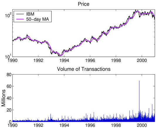
FIG. 1.: (top) IBM daily closing value signal between Jan. 01, 1990 and Dec. 31, 2000, i.e. 2780 data points with $yahoo$ moving averages for $\tau$ = 50 d; (bottom) daily volume of transactions in millions[11]

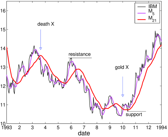
FIG. 2.: Typical IBM daily closing value signal between Jan. 01, 1993 and Dec. 31, 1993, with two moving averages, $M_{\tau_{1}}$ and $M_{\tau_{2}}$ for $\tau_{1}=5$ days and $\tau_{2}=21$ days. Death and gold crosses, resistance and support lines are defined in the text

FIG. 3.: pluses: density $\rho$ of crossing points between two moving averages with $\Delta\tau=(\tau_{1}-\tau_{2})/\tau_{2}$ and fixed $\tau_{2}=80$ from IBM daily closing value signal between Jan 01, 1990 and Dec 31, 2000; crosses : same for momentum indicators

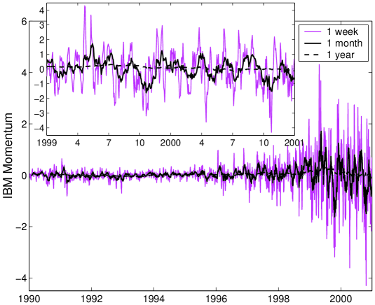
FIG. 4.: IBM 1 week, 1 month and 1 year $physical$ momentum between Jan. 01, 1990 and Dec. 31, 2000. Insert : blow up of the last two year time interval

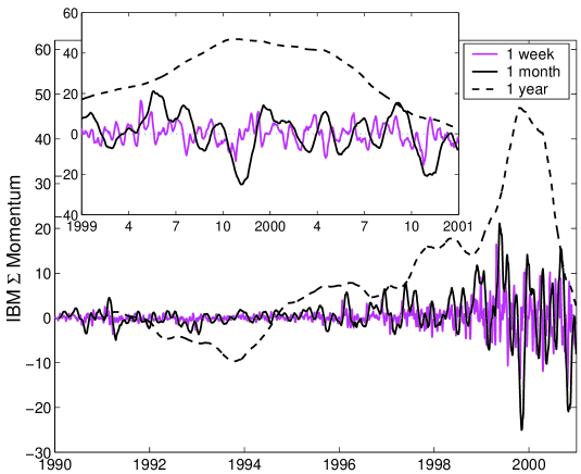
FIG. 5.: IBM momentum indicators for three different time periods $\tau$, 1 week (light gray curve), 1 month (gray curve) and 1 year (dash curve). Insert : blow up of the last two year time interval

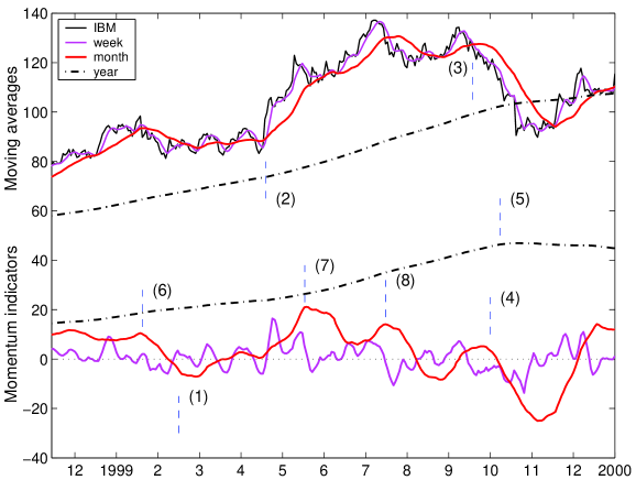
FIG. 6.: IBM signal, moving averages of IBM signal and its classical momentum indicators in 1999 or so for three time horizons, short-term (weekly) (light gray curve), medium-term (monthly) (gray curve) and log-term (yearly) (dot-dash curve), for discussing classical investment strategy; for lines at (1)-(5) see text

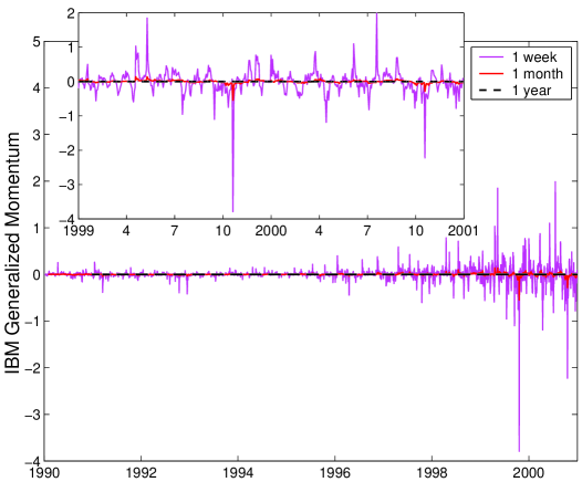
FIG. 7.: IBM generalized momentum between Jan 01, 1990 and Dec 31, 2000 for three different time periods $\tau$, 1 week (light gray curve), 1 month (gray curve) and 1 year (dash curve). Insert : blow up of the last two year time interval

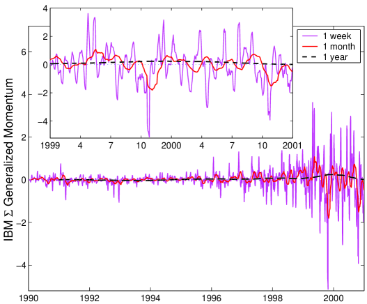
FIG. 8.: IBM generalized momentum indicators between Jan 01, 1990 and Dec 31, 2000 for three different time periods $\tau$, 1 week (light gray curve), 1 month (gray curve) and 1 year (dash curve). Insert : blow up of the last two year time interval

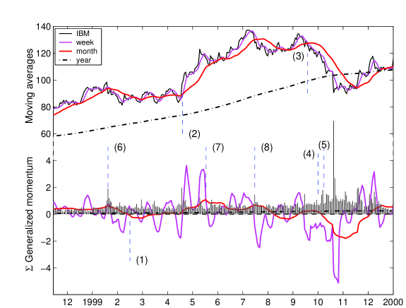
FIG. 9.: Volume of transactions (vertical lines), IBM signal, moving averages of IBM signal and its generalized momentum indicators in 1999 for three time horizons, short-term (weekly) (light gray curve), medium-term (monthly) (gray curve) and log-term (yearly) (dot-dash curve), for interpreting price evolution

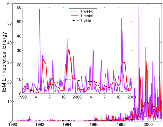
FIG. 10.: Theoretical (kinetic) energy of IBM between Jan 01, 1990 and Dec 31, 2000 for three time horizons, short-term (weekly) (light gray curve), medium-term (monthly) (gray curve) and log-term (yearly) (dot-dash curve); Insert : blow up of the last two year time interval

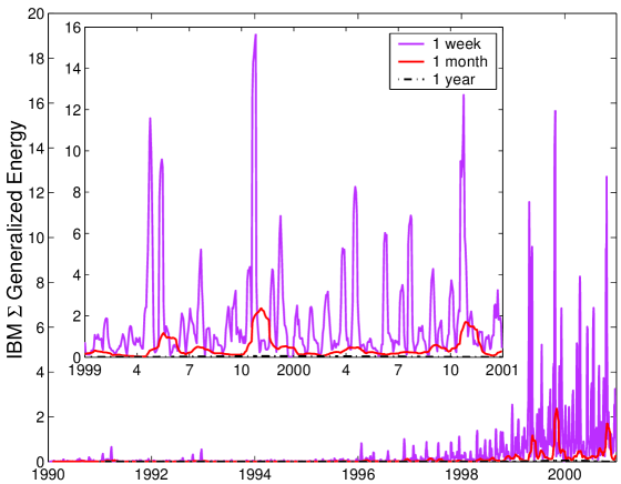
FIG. 11.: Generalized (kinetic) energy of IBM between Jan 01, 1990 and Dec 31, 2000 for three time horizons, short-term (weekly) (light gray curve), medium-term (monthly) (gray curve) and log-term (yearly) (dot-dash curve); Insert : blow up of the last two year time interval

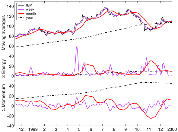
FIG. 12.: Comparison of moving averages, (kinetic) energy and momentum indicator of IBM in 1999 for three time horizons, short-term (weekly) (light gray curve), medium-term (monthly) (gray curve) and log-term (yearly) (dot-dash curve) in view of elaborating an investment strategy

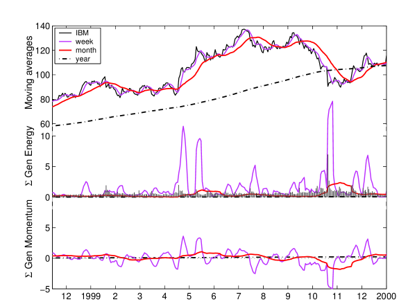
FIG. 13.: Comparison of moving averages, generalized (kinetic) energy and generalized momentum indicator of IBM in 1999 for three time horizons, short-term (weekly) (light gray curve), medium-term (monthly) (gray curve) and log-term (yearly) (dot-dash curve) in view of elaborating an investment strategy; the volume of transaction is displayed on the same line as the generalized energy

REFERENCES

- [1] see S.B. Achelis, in http://www.equis.com/free/taaz/
- [2] E.F. Fama, M. Blume, J. Bus. 39, 226 (1966)
- [3] F.E. James Jr., J. Financ. Quant. Anal. 3, 315 (1968)
- [4] W. Brock, J. Lakonishok, B. LeBaron, J. Finance 47, 1731 (1992)
- [5] R. Hudson, M. Dempsey, K. Keasey, J. Banking Finance 20, 1121 (1996)
- [6] A.C. Szakmary, I. Mathur, J. Int. Money Finance 16, 513 (1997)
- [7] F. Parisi, A.Vasquez, Emerging Markets Review 1, 152 (2000)
- [8] A.Gunasekarage, D. M. Power, Emerging Markets Review 2, 17 (2001)
- [9] K. Ivanova, Physica A 270, 567 (1999)
- [10] M. Ausloos, K. Ivanova, unpublished
- [11] http://finance.yahoo.com
- [12] N. Vandewalle, M. Ausloos, Ph. Boveroux Physica A 269, 170 (1999)
- [13] N. Vandewalle, M. Ausloos, Phy. Rev E 58, 6832 (1998)
- [14] M. Ausloos, Physica A 284, 385 (2000)
- [15] J.V. Andersen, S. Gluzman, D. Sornette, Eur. Phys. J. B 14, 579 (2000)
- [16] P. Gopikrishnan, V. Plerou, X. Gabaix, L.A.N. Amaral, H.E. Stanley, Physica A 299, 137 (2001)
- [17] F. Castiglione, R.B. Pandey, D. Stauffer,Physica A 289, 223 (2001)
- [18] W. M. Saslow, Am. J. Phys. 67, 1239 (1999)
- [19] J.G. de Gooijer, A. Klein, Intern. J. Forecast. 7, 501 (1992)