p-spin model in finite dimensions and its relation to structural glasses

Abstract

The p-spin spin-glass model has been studied extensively at mean-field level because of the insights which it provides into the mode-coupling approach to structural glasses and the nature of the glass transition. We demonstrate explicitly that the finite dimensional version of the p-spin model is in the same universality class as an Ising spin glass in a magnetic field. Assuming that the droplet picture of Ising spin glasses is valid we discuss how this universality may provide insights into why structural glasses are either “fragile” or “strong”.

In recent years structural glasses have been studied by many researchers using ideas from spin glasses. This activity was initiated by Kirkpatrick, Thirumalai and Wolynes Kirk who observed the similarity between the dynamical behavior of p-spin spin glass models at mean-field level and the mode-coupling equation for glasses Gotze . At mean-field level, the p-spin model has two transitions Bouchaud of interest for the structural glass analogy. There is a dynamical transition temperature $T_{d}$ below which the spin-spin correlation functions do not decay to zero in the long time limit which implies a breakdown of ergodicity. It is this transition which corresponds to the transition in the mode-coupling equations. The transition at $T_{c}<T_{d}$ is a transition associated with thermodynamic singularities (there are none at the dynamical transition $T_{d}$) and below it replica symmetry is broken at the “one-step” level Bouchaud . It is this transition which is usually identified with the glass transition (if any) of structural glasses and $T_{c}$ associated with, say, the Kauzmann temperature $T_{K}$ Kauzmann .

It has long been recognised that the dynamical transition at $T_{d}$ is an artifact of the mean-field limit Parisi ,Drossel . The transition is due to the exponentially large number of states which trap the system for exponentially long times forbidding the system in the thermodynamic limit from reaching equilibrium. However, in finite dimensional systems activation processes over finite free-energy barriers or nucleation processes will take place and restore ergodicity, a feature which was not incorporated either into the early versions of mode-coupling theory. Thus the type of transition which occurs at $T_{c}$ is the only possible transition which might exist in finite-dimensional p-spin models. In fact in this paper we will argue that this transition does not survive either in finite dimensional models of p-spin glasses. If the connection between real glasses and p-spin models goes beyond the mean-field limit then one would expect that there will be no genuine transition in real glasses either.

Our approach will be to start from a commonly used finite dimensional version of the p-spin model Parisi and study it using field-theoretic methods. We find that the field theory of the p-spin model (at least when p is three, the only value that we shall consider here) is in the same universality class as the Ising spin-glass in a magnetic field. The possibility of such a connection was suggested by Parisi et al. Parisi based on their numerical simulations and by Drossel et al. Drossel from their Migdal-Kadanoff renormalisation group studies, but it has never to our knowledge been explicitly demonstrated. While both models lack time reversal invariance, at mean-field level the p-spin model and the Ising spin glass in a magnetic field behave quite differently so that their similarity for finite dimensional systems cannot be taken as obvious. This is because the phase below $T_{c}$ in the mean-field p-spin model has replica symmetry broken at the one-step level Bouchaud , whereas the transition in the mean-field Ising spin-glass in a magnetic field – the transition discovered by de Almeida and Thouless (AT) AT ; BR – has the replica symmetry broken at all steps.

Away from the mean-field limit the existence of a transition for the Ising spin glass in a magnetic field remains controversial. According to the droplet picture BM ; FH ; McM , the presence of a field removes the phase transition just as a field applied to a ferromagnet does. However, advocates of the replica symmetry breaking picture of spin glasses claim that the AT transition exists in finite dimensions Marinari . In what follows we shall interpret our central result of the equivalence of the p-spin model with the Ising spin glass in a field according to the droplet model, and not discuss the consequences of this equivalence in the replica symmetry breaking picture. To support this interpretation we have determined the correlation length $\xi$ of the p-spin model as a function of the temperature $T$ using the Migdal-Kadanoff approximation (MKA) Drossel . The correlation length rises rapidly below a certain temperature before saturating at a large value, which is around 30 lattice spacings in three dimensions, but there is no evidence within this approach of an actual phase transition and a diverging correlation length.

In the three-spin model used for the present study, each site is occupied by two Ising spins, $\sigma_{i}$ and $\tau_{i}$, and the Hamiltonian is

$${\mathcal{H}}(\{\sigma\},\{\tau\})= - \sum_{<ij>}\left(J_{ij}^{(1)}\sigma_{i}\tau_{i}\sigma_{j}+J_{ij}^{(2)}\sigma_{i}\tau_{i}\tau_{j}\right.$$ (1)

$${}+\left.J_{ij}^{(3)}\sigma_{i}\sigma_{j}\tau_{j}+J_{ij}^{(4)}\tau_{i}\sigma_{j}\tau_{j}\right),$$

where ${<ij>}$ are nearest-neighbor pairs, and the couplings $J_{ij}^{(n)}$ are chosen independently from a Gaussian distribution with zero mean and width $J$.

When the signs of all the spins are reversed, the sign of the Hamiltonian changes, indicating the violation of time reversal symmetry. The thermal averages $\langle\sigma_{i}\rangle$ and $\langle\tau_{i}\rangle$ are non-zero at all finite temperatures.

In order to derive a field theory for the three-spin model we use the usual replica identity for the free energy $F$

$$F=-kT\overline{{\rm ln}(Z)}=-kT\lim_{n\rightarrow 0}\frac{\overline{Z^{n}}-1}{n}$$ (2)

to perform the average over the couplings $J_{ij}^{(n)}$, indicated by the overline. To evaluate $\overline{Z^{n}}$ we set up $n$ replicas of the partition function $Z$

$$Z^{n}={\rm Tr}\prod_{\alpha=1}^{n}\exp\left[-{\mathcal{H}}\left(\{\sigma^{\alpha}\},\{\tau^{\alpha}\}\right)/kT\right].$$ (3)

${\rm Tr}$ denotes taking the sum over the values $\pm 1$ of the Ising spins $\sigma_{i}^{\alpha}$ and $\tau_{i}^{\alpha}$ at each site. After bond averaging one gets

$$\overline{Z^{n}}={\rm Tr}\,\exp\bigg{[}\beta^{2}J^{2}nzN+\frac{1}{2}\beta^{2}J^{2}\sum_{<ij>}\sigma_{i}^{\alpha}\sigma_{i}^{\beta}\tau_{i}^{\alpha}\tau_{i}^{\beta}$$

$$\times\left(\sigma_{j}^{\alpha}\sigma_{j}^{\beta}+\tau_{j}^{\alpha}\tau_{j}^{\beta}\right)+\sigma_{j}^{\alpha}\sigma_{j}^{\beta}\tau_{j}^{\alpha}\tau_{j}^{\beta}\left(\sigma_{i}^{\alpha}\sigma_{i}^{\beta}+\tau_{i}^{\alpha}\tau_{i}^{\beta}\right)\bigg{]},$$ (4)

where $z$ is the number of neighbors of a site (six for a simple cubic lattice) and $N$ is the number of lattice sites.

The terms involving different sites are decoupled by introducing fields $q_{ij}^{\alpha\beta}$ and $p_{ij}^{\alpha\beta}$ for each bond $<ij>$ using:

$$\overline{Z^{n}}={\rm Tr}\,\exp\left(\beta^{2}J^{2}nzN\right)\prod_{<ij>}\frac{2}{\pi^{2}\beta^{4}J^{4}}\int d^{2}q_{ij}^{\alpha\beta}\int d^{2}p_{ij}^{\alpha\beta}$$ (5)

$$\times\exp\bigg{[}-\frac{\sqrt{2}}{\beta^{2}J^{2}}\left(q_{ij}^{\alpha\beta}q_{ij}^{\alpha\beta\ast}+p_{ij}^{\alpha\beta}p_{ij}^{\alpha\beta\ast}\right)$$

$${}+q_{ij}^{\alpha\beta}\sigma_{i}^{\alpha}\sigma_{i}^{\beta}\tau_{i}^{\alpha}\tau_{i}^{\beta}+{p_{ij}^{\alpha\beta}}\left(\sigma_{i}^{\alpha}\sigma_{i}^{\beta}+\tau_{i}^{\alpha}\tau_{i}^{\beta}\right)/\sqrt{2}$$

$${}+p_{ij}^{\alpha\beta\ast}\sigma_{j}^{\alpha}\sigma_{j}^{\beta}\tau_{j}^{\alpha}\tau_{j}^{\beta}+{q_{ij}^{\alpha\beta\ast}}\left(\sigma_{j}^{\alpha}\sigma_{j}^{\beta}+\tau_{j}^{\alpha}\tau_{j}^{\beta}\right)/\sqrt{2}\bigg{]},$$

where in the applied summation convention used here and in what follows for terms containing $\alpha$ and $\beta$ those for which $\alpha=\beta$ are to be omitted. We next follow the procedure of Pytte and Rudnick Pytte and define

$$Q_{\alpha\beta}(i)\equiv\sum_{j}q_{ij}^{\alpha\beta}\,$$

$$P_{\alpha\beta}(i)\equiv\sum_{j}p_{ij}^{\alpha\beta}.$$ (6)

We are left with the following types of sum at each site:

$${\rm Tr}\,\exp\left[Q_{\alpha\beta}(i)\sigma_{i}^{\alpha}\sigma_{i}^{\beta}\tau_{i}^{\alpha}\tau_{i}^{\beta}+\frac{P_{\alpha\beta}^{\ast}(i)}{\sqrt{2}}\left(\sigma_{i}^{\alpha}\sigma_{i}^{\beta}+\tau_{i}^{\alpha}\tau_{i}^{\beta}\right)\right].$$ (7)

These can be done by expanding the exponential, taking the trace and then re-exponentiating the result. Repeating this procedure for each site and finally taking the continuum limit one obtains, correct to $O(Q_{\alpha\beta}^{3},P_{\alpha\beta}^{3})$, the following free-energy density

$$\mathcal{F} = \frac{1}{4}{\nabla}Q_{\alpha\beta}{\nabla}Q_{\alpha\beta}^{\ast}+\frac{1}{4}{\nabla}P_{\alpha\beta}{\nabla}P_{\alpha\beta}^{\ast}+r\big{(}Q_{\alpha\beta}Q_{\alpha\beta}^{\ast}$$ (8)

$${}+P_{\alpha\beta}P_{\alpha\beta}^{\ast}\big{)}-a(Q_{\alpha\beta}^{2}+Q_{\alpha\beta}^{\ast 2}+P_{\alpha\beta}^{2}+P_{\alpha\beta}^{\ast 2})$$

$$- \frac{1}{6}\tilde{w}_{1}\left(Q_{\alpha\beta}Q_{\beta\gamma}Q_{\gamma\alpha}+Q_{\alpha\beta}^{\ast}Q_{\beta\gamma}^{\ast}Q_{\gamma\alpha}^{\ast}\sqrt{2}\right)$$

$$- \frac{1}{6}\tilde{w}_{1}\left(P_{\alpha\beta}P_{\beta\gamma}P_{\gamma\alpha}/\sqrt{2}+P_{\alpha\beta}^{\ast}P_{\beta\gamma}^{\ast}P_{\gamma\alpha}^{\ast}\right)$$

$$- \frac{1}{6}\tilde{w}_{2}\left(P_{\alpha\beta}^{2}Q_{\alpha\beta}+P_{\alpha\beta}^{\ast}Q_{\alpha\beta}^{\ast 2}\right),$$

where all fields have the symmetry $Q_{\alpha\beta}\equiv Q_{\beta\alpha}$, $\alpha\neq\beta$ and the implied summation convention is used. Notice that the free energy derived from the functional $\mathcal{F}$ is real as can be shown by taking the complex conjugate of Eq.(8) and making a variable change $P\Leftrightarrow Q$ in the fields, which are of course integrated over to get the free energy $F$.

The above field theory, while complicated, is of standard type. The field theory for the p-spin model obtained by Campellone et al. Campellone is very unusual and does not lend itself to a diagrammatic expansion. Truncating the expansion at the cubic terms is adequate provided that the phase transition, if any, is continuous. At mean-field level, the transition is continuous provided $w_{2}/w_{1}$ is sufficiently small (see below). The numerical studies of the three-spin model in finite dimensions suggest that the transition, if it exists, is continuous, so that we shall focus on situations in which the truncation to a cubic field theory is sufficient. When this is the case further simplifications are possible by simplifying the field theory to the soft modes associated with the possible transition.

First of all, it is easy to see from the quadratic terms that as the coefficient $a$ is positive the terms involving the imaginary parts of $Q$ and $P$ are associated with hard modes and so can all be dropped near the putative transition. The associated free energy density functional is then

$$\mathcal{F} = \frac{1}{4}({\nabla}A_{\alpha\beta})^{2}+\frac{1}{4}({\nabla}B_{\alpha\beta})^{2}-\frac{1}{4}t(A_{\alpha\beta}^{2}+B_{\alpha\beta}^{2})$$ (9)

$$- \frac{1}{6}w_{1}(A_{\alpha\beta}A_{\beta\gamma}A_{\gamma\alpha}+B_{\alpha\beta}B_{\beta\gamma}B_{\gamma\alpha})$$

$$- \frac{1}{6}w_{2}(A_{\alpha\beta}^{2}B_{\alpha\beta}+A_{\alpha\beta}B_{\alpha\beta}^{2}),$$

where $A_{\alpha\beta}$ is the real part of $Q_{\alpha\beta}$ and $B_{\alpha\beta}$ is the real part of $P_{\alpha\beta}$; $-t/4=(r-2a)$, $w_{1}=(1+1/\sqrt{2})\tilde{w}_{1}$, $w_{2}=\tilde{w}_{2}$. This functional is manifestly real.

A second simplification comes from observing that even at high temperatures $\langle A_{\alpha\beta}\rangle=\langle B_{\alpha\beta}\rangle\neq 0$, that is, the average of the fields is always non-zero. This is due to the term $(A_{\alpha\beta}^{2}B_{\alpha\beta}+A_{\alpha\beta}B_{\alpha\beta}^{2})$. Any transition which occurs will involve a breaking of this replica symmetric solution. It is convenient to first introduce the new fields

$$C_{\alpha\beta} = (A_{\alpha\beta}+B_{\alpha\beta})/\sqrt{2}$$

$$D_{\alpha\beta} = (A_{\alpha\beta}-B_{\alpha\beta})/\sqrt{2}.$$ (10)

Then in terms of these new fields the free energy functional becomes

$$\mathcal{F} = \frac{1}{4}({\nabla}C_{\alpha\beta})^{2}+\frac{1}{4}({\nabla}D_{\alpha\beta})^{2}-\frac{1}{4}t(C_{\alpha\beta}^{2}+D_{\alpha\beta}^{2})$$

$$- \frac{1}{6}v_{2}(C_{\alpha\beta}^{3}-C_{\alpha\beta}D_{\alpha\beta}^{2})-\frac{1}{6}v_{1}(C_{\alpha\beta}C_{\beta\gamma}C_{\gamma\alpha}$$

$$+ D_{\alpha\beta}D_{\beta\gamma}C_{\gamma\alpha}+D_{\alpha\beta}C_{\beta\gamma}D_{\gamma\alpha}+C_{\alpha\beta}D_{\beta\gamma}D_{\gamma\alpha}),$$

where $v_{1}=w_{1}/\sqrt{2}$ and $v_{2}=w_{2}/\sqrt{2}$. If one introduces a field $s_{\alpha\beta}$ such that $C_{\alpha\beta}=s_{\alpha\beta}+C$ with $<s_{\alpha\beta}>=0$ then one can see that the terms involving the $D_{\alpha\beta}$ fields are hard modes and can therefore be dropped. The free energy density functional is then

$$\mathcal{F}=\frac{1}{4}({\nabla}C_{\alpha\beta})^{2}-\frac{1}{4}tC_{\alpha\beta}^{2}-\frac{1}{6}v_{1}C_{\alpha\beta}C_{\beta\gamma}C_{\gamma\alpha}-\frac{1}{6}v_{2}C_{\alpha\beta}^{3}.$$ (12)

Ferrero et al. Ferrero wrote down this functional as the generic functional for discussing replica symmetry breaking at the one step level. They showed that the transition at mean-field level is continuous when $v_{2}/v_{1}\leq 1$.

The functional in terms of the $s_{\alpha\beta}$ fields (leaving out terms independent of $s_{\alpha\beta}$) is

$$\mathcal{F} = \frac{1}{4}({\nabla}s_{\alpha\beta})^{2}-\frac{1}{2}(t+v_{1}C^{2}+v_{2}C^{2})s_{\alpha\beta}$$ (13)

$$- \frac{1}{4}(t+2v_{2}C)s_{\alpha\beta}^{2}-\frac{1}{2}v_{1}Cs_{\alpha\beta}s_{\alpha\gamma}$$

$$- \frac{1}{6}v_{1}s_{\alpha\beta}s_{\beta\gamma}s_{\gamma\alpha}-\frac{1}{6}v_{2}s_{\alpha\beta}^{3},$$

where in the term $\frac{1}{2}v_{1}Cs_{\alpha\beta}s_{\alpha\gamma}$, $\beta\neq\gamma$. Writing the quadratic terms in the form

$$\frac{1}{4}({\nabla}s_{\alpha\beta})^{2}+M_{\alpha\beta,\gamma\delta}s_{\alpha\beta}s_{\gamma\delta},$$ (14)

it turns out that the matrix $\mathbf{M}$ has three distinct eigenvalues AT . The limit of stability of the replica symmetric high-temperature phase at mean-field level is determined by the vanishing of the smallest of these. AT showed that the corresponding eigenvectors span an $\frac{1}{2}n(n-3)$ dimensional subspace of the $\frac{1}{2}n(n-1)$ dimensional space defined by the $s_{\alpha\beta}$. This is called the “replicon subspace” BMR and since only the replicon modes go soft at the AT or replica symmetry breaking transition it suffices again to retain only these modes for a study of the critical behavior of this transition. It is useful to introduce the projection operator $S_{\alpha\beta,\gamma\delta}$ which projects any field $s_{\alpha\beta}$ onto the replicon subspace BR . Then $\tilde{q}_{\alpha\beta}=\sum S_{\alpha\beta,\gamma\delta}s_{\gamma\delta}$, where the sum is over distinct pairs $(\gamma\delta)$. The matrix elements are $S_{\alpha\beta,\alpha\beta}=3,S_{\alpha\beta,\alpha\gamma}=3/2,(\beta\neq\gamma)$ and $S_{\alpha\beta,\gamma\delta}=1,(\alpha,\beta,\gamma,\delta$ all different) when $n$ is set to zero. Then our final free energy density functional is

$$\mathcal{F}=\frac{1}{4}({\nabla}\tilde{q}_{\alpha\beta})^{2}+\frac{1}{4}\tilde{t}\tilde{q}_{\alpha\beta}^{2}-\frac{1}{6}v_{1}\tilde{q}_{\alpha\beta}\tilde{q}_{\beta\gamma}\tilde{q}_{\gamma\alpha}-\frac{1}{6}v_{2}\tilde{q}_{\alpha\beta}^{3},$$ (15)

where the coefficient $\tilde{t}$ is a measure of the distance from the transition (if any). Bray and Roberts BR first obtained this functional in their study of the critical exponents in dimension $6-\epsilon$ at the AT line.

Thus the ultimate field theory for the transition (if any) in the p-spin model is that of the Ising spin glass in a magnetic field. Bray and Roberts BR obtained the recursion equations for the coupling constants $v_{1}$ and $v_{2}$ correct to order $\epsilon$ but did not find any stable fixed point. They suggested that a possible explanation for this might be that there is no transition. We next provide some evidence using the Migdal-Kadanoff renormalisation group procedure that this indeed may be the correct interpretation of their perturbative renormalisation group calculation.

The MKA is a real-space renormalization method which we have previously applied Drossel to both the three-spin model and the Ising spin glass in a field. For both models the behavior of the couplings such as $J_{ij}^{(n)}$ under the renormalisation group was to flow to the high-temperature sink i.e. zero, implying that there was no transition. We have now investigated how the effective couplings decrease as a function of the lengthscale $L$ and find that the variance of $J_{ij}^{(n)}$ decreases as $\exp(-L/\xi)$, where $\xi(T)$ is the correlation length of the system. The dependence of $\xi(T)$ on temperature is shown in Figure 1 and it is obvious that because of the rapid rise of $\xi(T)$ when $T\approx 2J$ Monte Carlo numerical studies on systems of linear dimensions less than 10 could easily appear to have a phase transition Parisi .

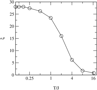
Figure 1: The correlation length of the three-spin model in three dimensions as function of $T/J$, as obtained using the MKA.

What can we deduce from these results on p-spin glasses for the physics of structural glasses? The connection of the transition at $T_{c}$ in the p-spin model (if any) with the structural glass transition at around $T_{K}$ (if any) has been much discussed Bouchaud . The relationship can really only go beyond an analogy if the two systems belong to the same universality class like, for example, the Ising ferromagnet and the liquid-gas critical point transition. At first sight any relationship between the p-spin model and phenomena in supercooled liquids seems unlikely. The p-spin model has quenched disorder, and there is no disorder at all in the glass transition problem. If there is a connection it would probably arise from similarities of the pure states in the two systems. The one-step replica symmetry broken state below $T_{c}$ implies that there are many pure states present each with the same overlap with each other Bouchaud . If a structural glass is formed via a phase transition it might have pure states with similar properties and then the functional of Eq. (15) might describe its transition correctly.

It is our contention though that there is no phase transition in the finite-dimensional p-spin model (in any finite dimension) and hence discussions of universality classes are not possible. However, the fact that a large correlation length can arise at low temperatures means that scaling and universality ideas should have a degree of utility and hence that the p-spin model may provide a qualitative model for structural glasses. According to this possibility one could argue that the more rapid growth than Arrhenius for the relaxation time $\tau$ seen in some glasses ( the “fragile” glasses) is because the relaxation time grows as

$$\tau=\tau_{0}\exp\left[B\xi(T)^{\psi}/kT\right]$$ (16)

accepting the connection to the droplet model of spin glasses, where $\tau_{0}$ is a microscopic relaxation time, and the constant $B$ would be expected to be of order $J$. The exponent $\psi$ would be that of the zero field Ising spin glass FH . The rapid rise of $\xi(T)$ depicted in Figure 1 would then produce a very non-Arrhenius temperature dependence of the relaxation time $\tau$. On the other hand some glasses (the “strong” glasses) do have an Arrhenius temperature dependence of their relaxation time. We would interpret this as arising when $\xi(T)$ at low temperatures is not large but instead of order one. It is our contention that the structural glass problem is similar to the Ising spin glass in a field, and if that field is large the correlation length is small BM ; Drossel and the non-Arrhenius behavior produced by a rapidly increasing correlation length will be absent in those circumstances. The validity of this picture would be greatly strengthened if experimental evidence of a growing correlation length at temperatures around $T_{K}$ in fragile glasses were to be experimentally observed.