Quantum field theory of dilute homogeneous Bose-Fermi
mixtures at zero temperature: general formalism
and beyond mean-field corrections

Abstract

We consider a dilute homogeneous mixture of bosons and spin-polarized fermions at zero temperature. We first construct the formal scheme for carrying out systematic perturbation theory in terms of single particle Green’s functions. We especially focus on the description of the boson-fermion interaction. To do so we need to introduce a new relevant object, the renormalized boson-fermion $T$-matrix which we determine to second order in the boson-fermion $s$-wave scattering length. We also discuss how to incorporate the usual boson-boson $T$-matrix in mean-field approximation to obtain the total ground state properties of the system. The next order term beyond mean-field stems from the boson-fermion interaction and is proportional to $a_{\mbox{BF}}k_{\mbox{F}}$. The total ground-state energy-density reads $E/V=\epsilon_{\mbox{F}}+\epsilon_{\mbox{B}}+(2\pi\hbar^{2}a_{\rm BF}n_{\mbox{B}}n_{\mbox{F}}/m)[1+a_{\mbox{BF}}k_{\mbox{F}}f(\delta)/\pi]$. The first term is the kinetic energy of the free fermions, the second term is the boson-boson mean-field interaction, the pre-factor to the additional term is the usual mean-field contribution to the boson-fermion interaction energy, and the second term in the square brackets is the second-order correction, where $f(\delta)$ is a known function of $\delta=(m_{\mbox{B}}-m_{\mbox{F}})/(m_{\mbox{B}}+m_{\mbox{F}})$. We also compute the bosonic and the fermionic chemical potentials, the compressibilities, and the modification to the induced fermion-fermion interaction. We discuss the behavior of the total ground-state energy and the importance of the beyond mean-field correction for various parameter regimes, in particular considering mixtures of ⁶Li and ⁷Li and of ³He and ⁴He. Moreover we determine the modification of the induced fermion-fermion interaction due to the beyond mean-field effects. We show that there is no effect on the depletion of the Bose condensate to first order in the boson-fermion scattering length $a_{\mbox{BF}}$.

I Introduction

Following the spectacular success in achieving Bose-Einstein condensation in trapped, dilute atomic gases in 1995 [1, 2, 3], there has been an explosion of experimental and theoretical activity on this newly accessible state of matter (for recent reviews focusing on different experimental and theoretical aspects see for instance [4, 5, 6, 7, 8]). More recently, there has been increasing interest and experimental activity also in quantum degenerate ultra-cold Fermi gases [9, 10, 11, 12, 13, 14], in particular because of the possibility of observing a BCS type transition in a dilute atomic gas [15, 16]. Dilute mixtures of ultra-cold gases of bosonic and fermionic atoms are also receiving increased attention, in particular because sympathetic cooling of the fermions by the bosons is an important means of their achieving quantum degeneracy [11, 12, 13, 14], and also because bosons can mediate an induced (attractive) fermion-fermion interaction [17]. Moreover mixtures of atomic ³He and ⁴He have become interesting in their own right after the recent achievement of Bose-Einstein condensation in metastable ⁴He [18, 19], as they could represent a bridge towards the understanding of superfluidity in helium.

Current analyses of dilute mixtures of ultra-cold atomic boson and fermion vapors are based on mean-field approximations. They include for example the work on stability considerations for homogeneous systems by Viverit et al. [17], and the calculation of density distributions and phase separation of trapped mixtures by Nygaard and Mølmer [20]. Some interesting effects have been studied by Bijlsma et al. [21], where an effective modification of the fermion-fermion scattering length, mediated by boson-fermion scattering processes, was determined. Pu et al. determined the phonon spectrum of the Bose condensate in a boson-fermion mixture at zero temperature [22].

Mean-field approaches have proved to be extremely useful in the theoretical and experimental study of Bose-Einstein condensed dilute atomic gases, and are likely to prove similarly useful for quantum degenerate mixed boson-fermion systems. It is nevertheless desirable to consider beyond mean-field effects, and under what circumstances they are likely to be most relevant. For pure (unpolarized) fermion [23, 24, 25] and pure boson [24, 25, 26, 27, 28, 29, 30, 31] systems, expansions of the ground-state energy, in terms of the small parameters $k_{\mbox{F}}a_{\mbox{FF}}$ and $\sqrt{n_{\mbox{B}}a_{\mbox{BB}}^{3}}$ ($k_{\mbox{F}}$ is the Fermi wavenumber, $n_{\mbox{B}}$ the boson density, $a_{\mbox{FF}}$ and $a_{\mbox{BB}}$ the fermion-fermion and boson-boson scattering lengths), are well established. These expansions go beyond mean-field approximations while still depending only on the $s$-wave scattering lengths. Although determined for homogeneous systems, the use of beyond mean-field corrections arising from consideration of such expansions may be readily extended to the experimentally relevant case of inhomogeneous trapped gases by application of the local density approximation. In general, the beyond mean-field corrections for the bosons are smaller than for the fermions, since the exponent of the small dimensionless parameter $n^{1/3}a$ ($n$ is the density parameter and $a$ the scattering length) is $1$ in the fermion case but $3/2$ in the boson case.

In the case of dilute fermions immersed in a Bose gas an expansion of the ground-state energy in terms of the small parameters $\sqrt{a_{\mbox{BB}}^{3}n_{\mbox{B}}}$ and $n_{\mbox{F}}/n_{\mbox{B}}$, where $n_{\mbox{F}}$ is the fermion density, was performed by Saam [32]. This was motivated by considering quantum-degenerate dilute gases as a model for the behavior of superfluid helium, where the assumption of $n_{\mbox{F}}/n_{\mbox{B}}$ as a small parameter is justified by the much greater natural occurrence of bosonic ⁴He compared to that of the fermionic ³He isotope.

Systems where there are vastly more bosons than fermions are certainly experimentally achievable in dilute atomic gases, and it can in fact be advantageous to have an excess of bosons in order to enhance sympathetic cooling [11]. However, there is in principle no a priori reason to confine theoretical analyses to such systems. In fact, in recent experiments [13, 14] the numbers of fermions and bosons are comparable. Thus motivated, in the present paper we derive a systematic perturbative expansion for the ground-state energy and other related relevant physical quantities for dilute Bose-Fermi mixtures at zero temperature and for arbitrary ratios of the boson and fermion densities. In this way we determine the lowest-order correction to mean-field in the case of weakly interacting bosons and spin-polarized fermions in terms of the the gas parameter $k_{\mbox{F}}a_{\mbox{BF}}$, where $a_{\mbox{BF}}$ is the boson-fermion $s$-wave scattering length. The ground-state energy thus derived can then be implemented, in local density approximation, as the energy functional for the study of the experimentally relevant case of trapped mixtures, in complete analogy with the pure bosonic and pure fermionic cases.

The plan of the paper is as follows. In Section II we introduce the basic Hamiltonian for a system of interacting bosons and spin-polarized fermions, expressed in its grand-canonical form after performing the Bogoliubov replacement. In Section III we define the one particle Green’s functions needed for a systematic field-theoretical analysis of the boson-boson and boson-fermion interactions, and we determine the associated Feynman rules. In Section IV we implement the perturbative expansion by introducing the boson-fermion self-energy and the renormalized boson-fermion $T$-matrix in ladder approximation and by solving the corresponding Bethe-Salpeter equation to second order in $k_{\mbox{F}}a_{\mbox{BF}}$. In Section V we exploit the results obtained in the previous Sections to compute some relevant physical quantities. In particular we provide the expression for the ground-state energy density to second order in the gas parameter, the bosonic and fermionic chemical potentials, the compressibilities, and the induced fermion-fermion interaction. We then compare the results thus obtained with actual and foreseeable experimental situations to assess the relative importance of higher-order corrections with respect to the mean-field results. In Section VI conclusions are drawn and some possible future developments are discussed.

II System

A Hamiltonian and ground-state energy

1 Many-body Hamiltonian

We consider a homogeneous mixture of interacting bosons and fermions, imposing periodic boundary conditions on a volume $V$. In complete generality there are thus boson-boson, boson-fermion, and fermion-fermion interactions to consider. However, for spin-polarized fermions, there is no $s$-wave scattering contribution to the fermion-fermion interaction [33]. The first non-vanishing contribution is due to $p$-wave scattering, which can generally be neglected when compared to the boson-boson and boson-fermion interactions, which are due to $s$-wave scattering. We thus take into account $s$-wave scattering between bosons, and between bosons and fermions only.

In second-quantized form, the Hamiltonian describing this situation is

$$\hat{H}=\hat{T}_{\mbox{B}}+\hat{T}_{\mbox{F}}+\hat{U}+\hat{V},$$ (1)

where

$$\hat{T}_{\mbox{B}} = \frac{\hbar^{2}}{2m_{\mbox{B}}}\int d^{3}{\mathbf{x}}{\mathbf{\nabla}}\hat{\Phi}^{\dagger}({\mathbf{x}})\cdot{\mathbf{\nabla}}\hat{\Phi}({\mathbf{x}}),$$ (2)

$$\hat{T}_{\mbox{F}} = \frac{\hbar^{2}}{2m_{\mbox{F}}}\int d^{3}{\mathbf{x}}{\mathbf{\nabla}}\hat{\Psi}^{\dagger}({\mathbf{x}})\cdot{\mathbf{\nabla}}\hat{\Psi}({\mathbf{x}}),$$ (3)

$$\hat{U} = \int\int d^{3}{\mathbf{x}}d^{3}{\mathbf{x}}^{\prime}\hat{\Phi}^{\dagger}({\mathbf{x}})\hat{\Psi}^{\dagger}({\mathbf{x}}^{\prime})U(|{\mathbf{x}}-{\mathbf{x}}^{\prime}|)\hat{\Psi}({\mathbf{x}}^{\prime})\hat{\Phi}({\mathbf{x}}),$$ (4)

$$\hat{V} = \frac{1}{2}\int\int d^{3}{\mathbf{x}}d^{3}{\mathbf{x}}^{\prime}\hat{\Phi}^{\dagger}({\mathbf{x}})\hat{\Phi}^{\dagger}({\mathbf{x}}^{\prime})V(|{\mathbf{x}}-{\mathbf{x}}^{\prime}|)\hat{\Phi}({\mathbf{x}}^{\prime})\hat{\Phi}({\mathbf{x}}),$$ (5)

and where $\hat{\Phi}({\mathbf{x}})$ is a bosonic field operator, $\hat{\Psi}({\mathbf{x}})$ is a fermionic field operator, and $m_{\mbox{B}}$ and $m_{\mbox{F}}$ are the respective masses of the bosons and fermions. For later reference we also define

$$\hat{H}_{0} = \hat{T}_{\mbox{B}}+\hat{T}_{\mbox{F}},$$ (6)

$$\hat{W} = \hat{U}+\hat{V}.$$ (7)

2 Mean field theory

It is straightforward to determine a zero-temperature mean field theory for $\hat{H}$ [20]. Employing the well-known Thomas-Fermi approximation, the mean field ground-state energy density is

$$\frac{E}{V}=\frac{3}{5}\frac{\hbar^{2}k_{\mbox{F}}^{2}}{2m_{\mbox{F}}}n_{\mbox{F}}+\frac{2\pi\hbar^{2}a_{\mbox{BF}}}{m}n_{\mbox{B}}n_{\mbox{F}}+\frac{2\pi\hbar^{2}a_{\mbox{BB}}}{m_{\mbox{B}}}n^{2}_{\mbox{B}},$$ (8)

where $m=m_{\mbox{F}}m_{\mbox{B}}/(m_{\mbox{F}}+m_{\mbox{B}})$ is the reduced mass, and $k_{\mbox{F}}=(6\pi^{2}n_{\mbox{F}})^{1/3}$ is the fermi wave-number [34]. In the case of a pure fermionic system, beyond mean-field corrections to the ground state energy-density are given by [23]:

$$\frac{E_{\mbox{F}}}{V}=\frac{3\hbar^{2}k_{F}^{2}}{5m_{\mbox{F}}}n_{\mbox{F}}\left[1+\frac{128}{15}k_{\mbox{F}}a_{\mbox{F}}+(k_{\mbox{F}}a_{\mbox{F}})^{2}+\ldots\right].$$ (9)

For pure bosons corrections to the ground state have been calculated by, e.g., Hugenholtz and Pines [28] and by Wu [29]. These corrections are obtained via a perturbative expansion in terms of the bosonic gas parameter $\sqrt{n_{\mbox{B}}a^{3}_{\mbox{BB}}}$. As already mentioned, this parameter is in general smaller than the fermionic gas parameter (see also Sec. V B). Our goal is thus to determine a general expression equivalent to Eq. (9), taking into account boson-fermion interactions, while neglecting corrections proportional to higher powers of the bosonic gas parameter.

B Bogoliubov replacement and grand-canonical Hamiltonian

In order to determine the energy functional to higher order than in Eq. (8), we will adopt a perturbative approach using one-particle Green’s functions, in a way essentially equivalent to the field-theoretical treatment of pure bosonic and fermionic systems [24, 25]. We thus first carry out the Bogoliubov replacement [35], where the condensate bosons are treated as a $c$-number field:

$$\hat{\Phi}({\mathbf{x}})=\sqrt{n_{0}}+\hat{\phi}({\mathbf{x}}),$$ (10)

where $n_{0}=N_{0}/V$ is the condensate density, and $N_{0}$ is the number of (condensate) atoms in the $k=0$ mode. This prescription breaks particle number conservation (see [36, 37, 38, 39] for alternative Bogoliubov replacements that preserve particle number conservation); average particle number conservation is assured by introducing the grand-canonical Hamiltonian

$$\hat{K}=\hat{H}-\mu_{\mbox{B}}\hat{N}_{\mbox{B}},$$ (11)

where $\mu_{\mbox{B}}$ is a Lagrange multiplier, to be identified with the boson chemical potential [25]. Substituting Eq. (10) into Eq. (11), the grand-canonical Hamiltonian reads:

$$\hat{K}=\hat{K}_{0}-\mu_{\mbox{B}}N_{0}+\hat{U}_{1}+\hat{U}_{2}+\hat{U}_{3}+\hat{V}_{1}+\hat{V}_{2}+\hat{V}_{3}+\hat{V}_{4}+\hat{V}_{5}+\hat{V}_{6}+\hat{V}_{7},$$ (12)

where

$$\hat{K_{0}}=\frac{\hbar^{2}}{2m_{\mbox{B}}}\int d^{3}{\mathbf{x}}{\mathbf{\nabla}}\hat{\phi}^{\dagger}({\mathbf{x}})\cdot{\mathbf{\nabla}}\hat{\phi}({\mathbf{x}})+\frac{\hbar^{2}}{2m_{\mbox{F}}}\int d^{3}{\mathbf{x}}{\mathbf{\nabla}}\hat{\Psi}^{\dagger}({\mathbf{x}})\cdot{\mathbf{\nabla}}\hat{\Psi}({\mathbf{x}})-\mu_{\mbox{B}}\int d^{3}{\mathbf{x}}\hat{\phi}^{\dagger}({\mathbf{x}})\hat{\phi}({\mathbf{x}}),$$ (13)

$$\hat{U}_{1} = n_{0}\int\int d^{3}{\mathbf{x}}d^{3}{\mathbf{x}}^{\prime}\hat{\Psi}^{\dagger}({\mathbf{x}}^{\prime})U(|{\mathbf{x}}-{\mathbf{x}}^{\prime}|)\hat{\Psi}({\mathbf{x}}^{\prime}),$$ (14)

$$\hat{U}_{2} = \sqrt{n_{0}}\int\int d^{3}{\mathbf{x}}d^{3}{\mathbf{x}}^{\prime}\hat{\Psi}^{\dagger}({\mathbf{x}}^{\prime})U(|{\mathbf{x}}-{\mathbf{x}}^{\prime}|)\hat{\Psi}({\mathbf{x}}^{\prime})\hat{\phi}({\mathbf{x}})+\mbox{h.c.},$$ (15)

$$\hat{U}_{3} = \int\int d^{3}{\mathbf{x}}d^{3}{\mathbf{x}}^{\prime}\hat{\phi}^{\dagger}({\mathbf{x}})\hat{\Psi}^{\dagger}({\mathbf{x}}^{\prime})U(|{\mathbf{x}}-{\mathbf{x}}^{\prime}|)\hat{\Psi}({\mathbf{x}}^{\prime})\hat{\phi}({\mathbf{x}}),$$ (16)

$$\hat{V}_{1} = \frac{1}{2}n_{0}^{2}\int\int d^{3}{\mathbf{x}}d^{3}{\mathbf{x}}^{\prime}V(|{\mathbf{x}}-{\mathbf{x}}^{\prime}|),$$ (17)

$$\hat{V}_{2} = n_{0}\sqrt{n_{0}}\int\int d^{3}{\mathbf{x}}d^{3}{\mathbf{x}}^{\prime}V(|{\mathbf{x}}-{\mathbf{x}}^{\prime}|)\hat{\phi}({\mathbf{x}})+\mbox{h.c.},$$ (18)

$$\hat{V}_{3} = \frac{1}{2}n_{0}\int\int d^{3}{\mathbf{x}}d^{3}{\mathbf{x}}^{\prime}V(|{\mathbf{x}}-{\mathbf{x}}^{\prime}|)\hat{\phi}({\mathbf{x}}^{\prime})\hat{\phi}({\mathbf{x}})+\mbox{h.c.},$$ (19)

$$\hat{V}_{4} = n_{0}\int\int d^{3}{\mathbf{x}}d^{3}{\mathbf{x}}^{\prime}\hat{\phi}^{\dagger}({\mathbf{x}})V(|{\mathbf{x}}-{\mathbf{x}}^{\prime}|)\hat{\phi}({\mathbf{x}}^{\prime}),$$ (20)

$$\hat{V}_{5} = n_{0}\int\int d^{3}{\mathbf{x}}d^{3}{\mathbf{x}}^{\prime}\hat{\phi}^{\dagger}({\mathbf{x}})V(|{\mathbf{x}}-{\mathbf{x}}^{\prime}|)\hat{\phi}({\mathbf{x}}),$$ (21)

$$\hat{V}_{6} = \sqrt{n_{0}}\int\int d^{3}{\mathbf{x}}d^{3}{\mathbf{x}}^{\prime}\hat{\phi}^{\dagger}({\mathbf{x}})V(|{\mathbf{x}}-{\mathbf{x}}^{\prime}|)\hat{\phi}({\mathbf{x}}^{\prime})\hat{\phi}({\mathbf{x}})+\mbox{h.c.},$$ (22)

$$\hat{V}_{7} = \frac{1}{2}\int\int d^{3}{\mathbf{x}}d^{3}{\mathbf{x}}^{\prime}\hat{\phi}^{\dagger}({\mathbf{x}})\hat{\phi}^{\dagger}({\mathbf{x}}^{\prime})V(|{\mathbf{x}}-{\mathbf{x}}^{\prime}|)\hat{\phi}({\mathbf{x}}^{\prime})\hat{\phi}({\mathbf{x}}).$$ (23)

III Systematic perturbation theory with Green’s functions

A Green’s functions: definitions

The boson ($B$) and fermion ($F$) Green’s functions for the boson-fermion system are defined as

$$iG_{\mbox{B}}({\mathbf{x}},t,{\mathbf{x}}^{\prime},t^{\prime}) = \langle\xi|T[\hat{\Phi}({\mathbf{x}},t)\hat{\Phi}^{\dagger}({\mathbf{x}}^{\prime},t^{\prime})]|\xi\rangle,$$ (24)

$$iG_{\mbox{F}}({\mathbf{x}},t,{\mathbf{x}}^{\prime},t^{\prime}) = \langle\xi|T[\hat{\Psi}({\mathbf{x}},t)\hat{\Psi}^{\dagger}({\mathbf{x}}^{\prime},t^{\prime})]|\xi\rangle,$$ (25)

where the time argument in $\hat{\Phi}({\mathbf{x}},t)$ and $\hat{\Psi}({\mathbf{x}},t)$ means they evolve according to Heisenberg’s equations of motion, $T$ denotes the time ordered product, and $|\xi\rangle$ is the ground state of $\hat{K}$ (we similarly define $|\xi_{0}\rangle$ to be the ground state of $\hat{K}_{0}$). We use the Bogoliubov replacement to write

$$iG_{\mbox{B}}({\mathbf{x}},t,{\mathbf{x}}^{\prime},t^{\prime})=n_{0}+iG_{\mbox{B}}^{\prime}({\mathbf{x}},t,{\mathbf{x}}^{\prime},t^{\prime}),$$ (26)

where

$$iG^{\prime}_{\mbox{B}}({\mathbf{x}},t,{\mathbf{x}}^{\prime},t^{\prime})=\langle\xi|T[\hat{\phi}({\mathbf{x}},t)\hat{\phi}^{\dagger}({\mathbf{x}}^{\prime},t^{\prime})]|\xi\rangle$$ (27)

is the propagator for the non-condensate bosons.

B Perturbative expansion

The Green’s functions can be evaluated in perturbation theory [25], where $\hat{W}$ is the perturbation to $\hat{K}_{0}$. Thus

$$iG^{\prime}_{\mbox{B}}({\mathbf{x}},t,{\mathbf{x}}^{\prime},t^{\prime}) = \frac{\sum_{n=0}^{\infty}i\tilde{G}_{\mbox{B}}^{(n)}({\mathbf{x}},t,{\mathbf{x}}^{\prime},t^{\prime})}{\sum_{n=0}^{\infty}\langle\xi_{0}|S^{(n)}|\xi_{0}\rangle},$$ (28)

$$iG_{\mbox{F}}({\mathbf{x}},t,{\mathbf{x}}^{\prime},t^{\prime}) = \frac{\sum_{n=0}^{\infty}i\tilde{G}_{\mbox{F}}^{(n)}({\mathbf{x}},t,{\mathbf{x}}^{\prime},t^{\prime})}{\sum_{n=0}^{\infty}\langle\xi_{0}|S^{(n)}|\xi_{0}\rangle},$$ (29)

where

$$i\tilde{G}_{\mbox{B}}^{(n)}({\mathbf{x}},t,{\mathbf{x}}^{\prime},t^{\prime}) = \langle\xi_{0}|T[S^{(n)}\tilde{\phi}({\mathbf{x}},t)\tilde{\phi}^{\dagger}({\mathbf{x}}^{\prime},t^{\prime})]|\xi_{0}\rangle,$$ (30)

$$i\tilde{G}_{\mbox{F}}^{(n)}({\mathbf{x}},t,{\mathbf{x}}^{\prime},t^{\prime}) = \langle\xi_{0}|T[S^{(n)}\tilde{\Psi}({\mathbf{x}},t)\tilde{\Psi}^{\dagger}({\mathbf{x}}^{\prime},t^{\prime})]|\xi_{0}\rangle,$$ (31)

$$S^{(n)} = \frac{1}{n!}\left(\frac{-i}{\hbar}\right)^{n}\int dt_{1}\ldots\int dt_{n}T[\tilde{W}(t_{1})\ldots\tilde{W}(t_{n})].$$ (32)

Operators with a tilde are defined to be in the interaction picture, i.e. $\tilde{O}(t)=\exp(i\hat{K}_{0}t/\hbar)\hat{O}\exp(-i\hat{K}_{0}t/\hbar)$. In the limit of a non-interacting system ($\hat{W}\rightarrow 0$) the Green’s functions reduce to the zeroth order terms in the expansions, so that

$$iG_{\mbox{B}}^{0}({\mathbf{x}},t,{\mathbf{x}}^{\prime},t^{\prime}) = i\tilde{G}_{\mbox{B}}^{(0)}({\mathbf{x}},t,{\mathbf{x}}^{\prime},t^{\prime})=\langle\xi_{0}|T[\tilde{\phi}({\mathbf{x}},t)\tilde{\phi}^{\dagger}({\mathbf{x}}^{\prime},t^{\prime})]|\xi_{0}\rangle,$$ (33)

$$iG_{\mbox{F}}^{0}({\mathbf{x}},t,{\mathbf{x}}^{\prime},t^{\prime}) = i\tilde{G}_{\mbox{F}}^{(0)}({\mathbf{x}},t,{\mathbf{x}}^{\prime},t^{\prime})=\langle\xi_{0}|T[\tilde{\Psi}({\mathbf{x}},t)\tilde{\Psi}^{\dagger}({\mathbf{x}}^{\prime},t^{\prime})]|\xi_{0}\rangle.$$ (34)

C Evaluation of terms using Wick’s theorem

Equations (30), (31), and (32) can be evaluated by Wick’s theorem, which states that the vacuum (non-interacting ground-state) expectation values of time ordered products of operators can be expressed as the sum of all products of contractions of pairs of operators in the time-ordered product [40]. The contraction of two operators is defined as

$$\tilde{O}(t)^{(i)}\tilde{P}(t^{\prime})^{(i)}=T[\tilde{O}(t)\tilde{P}(t^{\prime})]\,-\,:\tilde{O}(t)\tilde{P}(t^{\prime}):\,,$$ (35)

where $:\tilde{O}(t)\tilde{P}(t^{\prime}):$ is the normal ordered product. In particular,

$$\tilde{\phi}({\mathbf{x}},t)^{(i)}\tilde{\phi}^{\dagger}({\mathbf{x}}^{\prime},t^{\prime})^{(i)} = \tilde{\phi}^{\dagger}({\mathbf{x}}^{\prime},t^{\prime})^{(i)}\tilde{\phi}({\mathbf{x}},t)^{(i)}=iG_{\mbox{B}}^{0}({\mathbf{x}},t,{\mathbf{x}}^{\prime},t^{\prime}),$$ (36)

$$\tilde{\Psi}({\mathbf{x}},t)^{(i)}\tilde{\Psi}^{\dagger}({\mathbf{x}}^{\prime},t^{\prime})^{(i)} = -\tilde{\Psi}^{\dagger}({\mathbf{x}}^{\prime},t^{\prime})^{(i)}\tilde{\Psi}({\mathbf{x}},t)^{(i)}=iG_{\mbox{F}}^{0}({\mathbf{x}},t,{\mathbf{x}}^{\prime},t^{\prime}),$$ (37)

and all other contractions of pairs of operators $\in\{\tilde{\phi}({\mathbf{x}},t),\tilde{\phi}^{\dagger}({\mathbf{x}}^{\prime},t^{\prime}),\tilde{\Psi}({\mathbf{x}}^{\prime\prime},t^{\prime\prime}),\tilde{\Psi}^{\dagger}({\mathbf{x}}^{\prime\prime\prime},t^{\prime\prime\prime})\}$ vanish (see also Appendix A). Substituting Eqs. (36) and (37) into Eqs. (30), (31), and (32), the first order terms can be determined to be:

$$i\tilde{G}_{\mbox{B}}^{(1)}(x^{\mu},y^{\mu}) = \frac{-i}{\hbar}\int\int d^{4}x_{1}^{\mu}d^{4}y_{1}^{\mu}\biggl{\{}U(x_{1}^{\mu}-y_{1}^{\mu})$$ (43)

$$\times\left[-n_{0}iG^{0}_{\mbox{F}}(y_{1}^{\mu},y_{1}^{\mu})iG^{0}_{\mbox{B}}(x^{\mu},y^{\mu})\right.$$

$$\left.-iG^{0}_{\mbox{F}}(y_{1}^{\mu},y_{1}^{\mu})iG^{0}_{\mbox{B}}(x^{\mu},x_{1}^{\mu})iG^{0}_{\mbox{B}}(x_{1}^{\mu},y^{\mu})\right]$$

$$+V(x_{1}^{\mu}-y_{1}^{\mu})\biggl{[}\frac{n_{0}^{2}}{2}iG^{0}_{\mbox{B}}(x^{\mu},y^{\mu})$$

$$+n_{0}iG^{0}_{\mbox{B}}(x^{\mu},x_{1}^{\mu})iG^{0}_{\mbox{B}}(x_{1}^{\mu},y^{\mu})$$

$$+n_{0}iG^{0}_{\mbox{B}}(x^{\mu},x_{1}^{\mu})iG^{0}_{\mbox{B}}(x^{\mu},x_{2}^{\mu})\biggr{]}\biggr{\}},$$

$$i\tilde{G}_{\mbox{F}}^{(1)}(x^{\mu},y^{\mu}) = \frac{-i}{\hbar}\int\int d^{4}x_{1}^{\mu}d^{4}y_{1}^{\mu}\biggl{\{}U(x_{1}^{\mu}-y_{1}^{\mu})$$ (47)

$$\times[-n_{0}iG^{0}_{\mbox{F}}(y_{1}^{\mu},y_{1}^{\mu})iG^{0}_{\mbox{F}}(x^{\mu},y^{\mu})$$

$$-n_{0}iG^{0}_{\mbox{F}}(x^{\mu},y_{1}^{\mu})iG^{0}_{\mbox{F}}(y_{1}^{\mu},y^{\mu})]$$

$$+V(x_{1}^{\mu}-y_{1}^{\mu})\frac{n_{0}^{2}}{2}iG_{\mbox{F}}(x^{\mu},y^{\mu})\biggr{\}}$$

$$S^{(1)} = \frac{-i}{\hbar}\int\int d^{4}x_{1}^{\mu}d^{4}y_{1}^{\mu}\biggl{\{}U(x_{1}^{\mu}-y_{1}^{\mu})$$ (49)

$$\times[-in_{0}G^{0}_{\mbox{F}}(y_{1}^{\mu},y_{1}^{\mu})]+V(x_{1}^{\mu}-y_{1}^{\mu})\frac{n_{0}^{2}}{2}\biggr{\}},$$

where we have used the more compact four-vector notation [$x^{\mu}=(t,{\mathbf{x}})$], and defined $U(x^{\mu}-y^{\mu})=U({\mathbf{x}}-{\mathbf{y}})\delta(x^{0}-y^{0})$ and $V(x^{\mu}-y^{\mu})=V({\mathbf{x}}-{\mathbf{y}})\delta(x^{0}-y^{0})$. Note that $G^{0}_{\mbox{B}}(t,{\mathbf{x}},t,{\mathbf{y}})=0$ (i.e. there are no boson loops at zero temperature).

Higher order terms may be similarly evaluated, and will similarly be expressed in terms of integrals over products of noninteracting Green’s functions, condensate factors $n_{0}$, and interaction terms. We represent these graphically (see Fig. 1): straight lines for fermions, wiggly lines for non-condensate bosons, dashed lines for condensate bosons, and zigzag lines for interaction terms (whether it is a boson-boson or boson-fermion interaction is clearly determined by the kinds of particle lines attached to the vertices of the interaction line):

FIG. 1.: Definition of the diagram lines

As is usual [24, 25, 41], all disconnected graphs in the numerator can be factorized out by the denominator, so that

$$G^{\prime}_{\mbox{B}}(x^{\mu},y^{\mu}) = \sum_{n=0}^{\infty}\tilde{G}_{\mbox{B}}^{(n)}(x^{\mu},y^{\mu})_{\mbox{connected}}\;,$$ (50)

$$G_{\mbox{F}}(x^{\mu},y^{\mu}) = \sum_{n=0}^{\infty}\tilde{G}_{\mbox{F}}^{(n)}(x^{\mu},y^{\mu})_{\mbox{connected}}\;.$$ (51)

Noting that each connected graph essentially appears $n!$ times, with simple permutations on the labeling, when composing such graphs we integrate over all internal variables and affix a factor of $(i/\hbar)^{n}(-1)^{F}(-i)^{C}$, where $n$ is the number of interaction lines, $F$ is the number of closed fermion loops, and $C$ is the number of dashed boson lines.

D Feynman rules

For homogeneous systems it is convenient to Fourier transform to energy-momentum space, so that:

$$G^{0}_{\mbox{B}}(p^{\mu}) = \frac{1}{p^{0}-\hbar p^{2}/2m_{\mbox{B}}+\mu_{B}/\hbar+i\nu},$$ (52)

$$G^{0}_{\mbox{F}}(p^{\mu}) = \frac{1}{p^{0}-\hbar p^{2}/2m_{\mbox{F}}+i\mbox{sgn}(p-k_{\mbox{F}})\nu},$$ (53)

where $\mbox{sgn}(k)=1$ for $k\geq 0$ and $=-1$ for $k<0$ (we write $p$ for $|\mathbf{p}|$). The appropriate Feynman rules for the boson (fermion) Green’s function in this representation are then:

1) Draw all topologically distinct connected diagrams with one outgoing external wiggly boson (fermion) line and one incoming external wiggly boson (fermion) line, no external fermion (boson) lines and no internal dashed boson lines, $n$ zigzag interaction lines, each of which is attached at one vertex to an incoming and an outgoing boson line (either wiggly or dashed), and at the other vertex either to an incoming and an outgoing boson line, or to an incoming and an outgoing (not necessarily distinct) fermion line. Each vertex must be attached to exactly one zigzag interaction line.

2) All wiggly boson lines must run into the same direction and there are no closed boson loops.

3) Each dashed boson line corresponds to a factor of $\sqrt{n_{0}}$, each wiggly boson line to a factor of $G^{0}_{\mbox{B}}(k^{\mu})$, each fermion line to a factor of $G^{0}_{\mbox{F}}(k^{\mu})$, each boson-fermion interaction line to a factor of $U(k^{\mu})=U({\mathbf{k}})$, and each boson-boson interaction line to a factor of $V(k^{\mu})=V({\mathbf{k}})$.

4) Assign a direction to each interaction line; associate a directed four-momentum with each line and conserve four-momentum at each vertex. Each dashed boson line carries four-momentum $0$ and each wiggly boson line has four-momentum $\neq 0$.

5) Integrate over the $n$ independent four-momenta.

6) Affix a factor of $(i/\hbar)^{n}(2\pi)^{-4(n)}(-1)^{F}(-i)^{C}$, where $F$ is the number of closed fermion loops and $C$ is the number of dashed boson lines.

IV Determination of the boson-fermion $T$-matrix and self-energies in ladder approximation

A The Hugenholtz-Pines theorem

According to the Hugenholtz-Pines theorem [28, 42], the bosonic chemical potential $\mu_{\mbox{B}}$, defined as

$$\frac{\partial E/V}{\partial n_{\mbox{B}}}=\mu_{\mbox{B}},$$ (54)

is given by

$$\mu_{\mbox{B}} = \hbar\Sigma_{\mbox{B}}(0)-\hbar\Sigma_{12}(0),$$ (55)

where $\Sigma_{\mbox{B}}(0)$ and $\Sigma_{12}(0)$ are the proper self-energies for the bosons due to their interaction with both bosons and fermions, evaluated at $p^{\mu}=0$ (in what follows we call them the bosonic self-energies). The self-energies are in general related to the Green’s functions by the Dyson equations. The Dyson equation for the bosons is given by:

$$\left(\begin{array}[]{cc}G_{\mbox{B}}^{\prime}(p^{\mu})&G_{12}(-p^{\mu})\\ G_{21}(p^{\mu})&G_{\mbox{B}}^{\prime}(-p^{\mu})\end{array}\right)=\left(\begin{array}[]{cc}G_{\mbox{B}}^{0}(p^{\mu})&0\\ 0&G_{\mbox{B}}^{0}(-p^{\mu})\end{array}\right)$$ (60)

(61)

$$+\left(\begin{array}[]{cc}G_{\mbox{B}}^{0}(p^{\mu})&0\\ 0&G_{\mbox{B}}^{0}(-p^{\mu})\end{array}\right)\left(\begin{array}[]{cc}\Sigma_{\mbox{B}}(p^{\mu})&\Sigma_{12}(p^{\mu})\\ \Sigma_{21}(p^{\mu})&\Sigma_{\mbox{B}}(-p^{\mu})\end{array}\right)\left(\begin{array}[]{cc}G_{\mbox{B}}^{\prime}(p^{\mu})&G_{12}(p^{\mu})\\ G_{21}(p^{\mu})&G_{\mbox{B}}^{\prime}(-p^{\mu})\end{array}\right)\;,$$ (68)

where have introduced the anomalous boson Green’s functions $G_{12}(p^{\mu})$ and $G_{21}(p^{\mu})$ (defined as the Fourier transforms of $G_{12}(x^{\mu},y^{\mu})=\langle\xi|T[\hat{\phi}(x^{\mu})\hat{\phi}(y^{\mu})]|\xi\rangle$ and $G_{21}(x^{\mu},y^{\mu})=\langle{\bf G}|[\hat{\phi}^{\dagger}(x^{\mu})\hat{\phi}^{\dagger}(y^{\mu})]|\xi\rangle$, respectively). The Dyson equation for the fermions takes the much simpler scalar form:

$$G_{\mbox{F}}(p^{\mu})=G_{\mbox{F}}^{0}(p^{\mu})+G_{\mbox{F}}^{0}(p^{\mu})\Sigma_{\mbox{F}}(p^{\mu})G_{\mbox{F}}(p^{\mu})\;,$$ (69)

where $\Sigma_{\mbox{F}}(p^{\mu})$ is the proper self-energy for the fermions due to the interaction with the bosons (the fermionic self-energy).

B The self-energies in ladder approximation

As we are considering a dilute system, in terms of Feynman diagrams only diagrams with interaction lines between two systems of connected propagators are important [24, 25] (ladder approximation). This is expressed in terms of the boson-fermion and boson-boson $T$-matrices in Fig. 2, where the boson-fermion $T$-matrix $T_{\mbox{BF}}$ in ladder approximation is defined in Fig. 3, the boson-boson $T$-matrix $T_{\mbox{BB}}$ (also in ladder approximation) is well known from studies of dilute pure Bose systems, and the normal (diagonal) bosonic proper self-energy is given by

$$\Sigma_{\mbox{B}}(p^{\mu})=\Sigma_{\mbox{BF}}(p^{\mu})+\Sigma_{\mbox{BB}}(p^{\mu}).$$ (70)

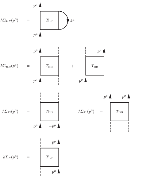
FIG. 2.: The self-energies in ladder approximation, expressed in terms of the $T$-matrices.

The proper self-energies can thus be determined by adding the proper self-energies of a system of interacting bosons to those of a hypothetical mixed boson-fermion system where there are boson-fermion interactions only [43]. This result arises from our use of the ladder approximation, and is not in general true (there also exist, for example, inseparable three-legged “ladders” consisting of a boson-boson and a boson-fermion ladder joined by a common boson leg, but these clearly involve three-particle processes). For such a hypothetical mixed system, the only self-energies we need to consider and to evaluate are $\Sigma_{\mbox{BF}}(p^{\mu})$ and $\Sigma_{\mbox{F}}(p^{\mu})$, which can be written algebraically as:

$$\hbar\Sigma_{\mbox{BF}}(p^{\mu}) = -\frac{i}{(2\pi)^{4}}\int d^{4}k^{\mu}T_{\mbox{BF}}(p^{\mu},k^{\mu},p^{\mu},k^{\mu})G^{0}_{\mbox{F}}(k^{\mu}),$$ (71)

$$\hbar\Sigma_{\mbox{F}}(p^{\mu}) = T_{\mbox{BF}}(0,p^{\mu},0,p^{\mu})n_{0}.$$ (72)

FIG. 3.: The boson-fermion $T$-matrix.

C Bethe-Salpeter equation for $T_{\mbox{BF}}$

FIG. 4.: The integral equation for $T_{\mbox{BF}}$.

The boson-fermion $T$-matrix $T_{\mbox{BF}}$ can also be represented recursively, as shown in Fig. 4. If we now transform to center-of-mass coordinates,

$$P^{\mu} = p_{1}^{\mu}+p_{2}^{\mu}=p_{3}^{\mu}+p_{4}^{\mu},$$ (73)

$$k_{1}^{\mu} = (p_{1}^{\mu}-p_{2}^{\mu})/2,$$ (74)

$$k_{2}^{\mu} = (p_{3}^{\mu}-p_{4}^{\mu})/2,$$ (75)

the algebraic form of the equation represented in Fig. 4 reads:

$$T_{\mbox{BF}}(k_{1}^{\mu},k_{2}^{\mu},P^{\mu}) = U({\mathbf{k}}_{1}-{\mathbf{k}}_{2})+\frac{i}{\hbar(2\pi)^{4}}\int d^{3}{\mathbf{k}}U({\mathbf{k}}_{1}-{\mathbf{k}})$$ (77)

$$\times\int dk^{0}G^{0}_{\mbox{B}}(P^{\mu}/2+k^{\mu})G^{0}_{\mbox{F}}(P^{\mu}/2-k^{\mu})T_{\mbox{BF}}(k^{\mu},k_{2}^{\mu},P^{\mu})\;.$$

This is a kind of Bethe-Salpeter integral equation, which we will now solve recursively for low momenta, stopping at order $a_{\mbox{BF}}^{2}$ . As the interactions are instantaneous, the only frequency dependence in $T_{\mbox{BF}}(k_{1}^{\mu},k_{2}^{\mu},P^{\mu})$ is in $P^{0}$ [24, 25]. Thus, a contour integration over $k^{0}$ in Eq. (77) yields:

$$T_{\mbox{BF}}({\mathbf{k}}_{1},{\mathbf{k}}_{2},P^{\mu})=U({\mathbf{k}}_{1}-{\mathbf{k}}_{2})$$ (78)

$$+\frac{1}{(2\pi)^{3}}\int d^{3}{\mathbf{k}}\frac{U({\mathbf{k}}_{1}-{\mathbf{k}})T_{\mbox{BF}}({\mathbf{k}},{\mathbf{k}}_{2},P^{\mu})\theta(|{\mathbf{P}}/2-{\mathbf{k}}|-k_{\mbox{F}})}{\hbar P^{0}-\hbar^{2}({\mathbf{P}}/2+{\mathbf{k}})^{2}/2m_{\mbox{B}}-\hbar^{2}({\mathbf{P}}/2-{\mathbf{k}})^{2}/2m_{\mbox{F}}+\mu+i\nu}.$$ (79)

We now express Eq. (79) in terms of the free scattering amplitude $f({\mathbf{k}}_{1},{\mathbf{k}}_{2})$, first by formally inversion (see [24]):

$$\frac{2\pi\hbar^{2}}{m}f({\mathbf{k}}_{1},{\mathbf{k}}_{2}) = U({\mathbf{k}}_{2}-{\mathbf{k}}_{1})+\frac{1}{(2\pi)^{3}}\int d^{3}{\mathbf{k}}\frac{U({\mathbf{k}}_{2}-{\mathbf{k}})2\pi\hbar^{2}f({\mathbf{k}}_{1},{\mathbf{k}})/m}{\hbar^{2}{\mathbf{k}}_{1}^{2}/2m-\hbar^{2}{\mathbf{k}}^{2}/2m+i\nu}\;,$$ (80)

and then by exploiting the resulting expression to rewrite Eq. (79) as:

$$T_{\mbox{BF}}({\mathbf{k}}_{1},{\mathbf{k}}_{2},P^{\mu}) = \frac{2\pi\hbar^{2}}{m}f({\mathbf{k}}_{2},{\mathbf{k}}_{1})+\frac{1}{(2\pi)^{3}}\int d^{3}{\mathbf{k}}\frac{2\pi\hbar^{2}}{m}f({\mathbf{k}},{\mathbf{k}}_{1})T_{\mbox{BF}}({\mathbf{k}},{\mathbf{k}}_{2},P^{\mu})$$ (83)

$$\times\left[\frac{\theta(|{\mathbf{P}}/2-{\mathbf{k}}|-k_{\mbox{F}})}{\hbar P^{0}-\hbar^{2}({\mathbf{P}}/2+{\mathbf{k}})^{2}/2m_{\mbox{B}}-\hbar^{2}({\mathbf{P}}/2-{\mathbf{k}})^{2}/2m_{\mbox{F}}+\mu+i\nu}\right.$$

$$\left.-\frac{1}{\hbar^{2}{\mathbf{k}}_{1}^{2}/2m-\hbar^{2}{\mathbf{k}}^{2}/2m+i\nu}\right]\,.$$

For low momenta the vacuum scattering amplitude $f({\mathbf{k}}_{1},{\mathbf{k}}_{2})$ can be expanded to second order in the scattering length $a_{\mbox{BF}}$ (see [25]):

$$f({\mathbf{k}}_{1},{\mathbf{k}}_{2})\approx a_{\mbox{BF}}-ia_{\mbox{BF}}^{2}k,$$ (84)

where $k=k_{1}=k_{2}\rightarrow 0$. We insert this into Eq. (83), iteratively substituting Eq. (83) into itself, and consistently keeping terms up to quadratic order in $a_{\mbox{BF}}$ only. This produces

$$T_{\mbox{BF}}({\mathbf{k}}_{1},{\mathbf{k}}_{2},P^{\mu}) \approx \frac{2\pi\hbar^{2}}{m}[a_{\mbox{BF}}-ia_{\mbox{BF}}^{2}k_{1}]+\frac{4\pi^{2}\hbar^{4}a_{\mbox{BF}}^{2}}{(2\pi)^{3}m^{2}}$$ (87)

$$\times\int d^{3}{\mathbf{k}}\left[\frac{\theta(|{\mathbf{P}}/2-{\mathbf{k}}|-k_{\mbox{F}})}{\hbar P^{0}-\hbar^{2}({\mathbf{P}}/2+{\mathbf{k}})^{2}/2m_{\mbox{B}}-\hbar^{2}({\mathbf{P}}/2-{\mathbf{k}})^{2}/2m_{\mbox{F}}+\mu+i\nu}\right.$$

$$\left.-\frac{1}{\hbar^{2}{\mathbf{k}}_{1}^{2}/2m-\hbar^{2}{\mathbf{k}}^{2}/2m+i\nu}\right],$$

the renormalized second order expansion of the boson-fermion $T$-matrix. The integral can be evaluated (see App. B) to give

$$T_{\mbox{BF}}({\mathbf{k}}_{1},{\mathbf{k}}_{2},P^{\mu})\approx\frac{2\pi\hbar^{2}}{m}a_{\mbox{BF}}+\frac{2\hbar^{2}a_{\mbox{BF}}^{2}k_{\mbox{F}}}{m}$$ (88)

(89)

$$+\frac{a_{\mbox{BF}}^{2}\hbar^{2}}{2m^{2}}\left(\frac{m_{\mbox{B}}k_{\mbox{F}}^{2}}{P}-\frac{m^{2}P}{m_{\mbox{B}}}-2m\sqrt{D}-\frac{m_{\mbox{B}}D}{P}\right)\ln\frac{k_{\mbox{F}}+mP/m_{\mbox{B}}+\sqrt{D}+i\nu/2a_{\mbox{BF}}\sqrt{D}}{k_{\mbox{F}}-mP/m_{\mbox{B}}-\sqrt{D}-i\nu/2a_{\mbox{BF}}\sqrt{D}}$$ (90)

(91)

$$-\frac{a_{\mbox{BF}}^{2}\hbar^{2}}{2m^{2}}\left(\frac{m_{\mbox{B}}k_{\mbox{F}}^{2}}{P}-\frac{m^{2}P}{m_{\mbox{B}}}+2m\sqrt{D}-\frac{m_{\mbox{B}}D}{P}\right)\ln\frac{k_{\mbox{F}}-mP/m_{\mbox{B}}+\sqrt{D}+i\nu/2a_{\mbox{BF}}\sqrt{D}}{k_{\mbox{F}}+mP/m_{\mbox{B}}-\sqrt{D}-i\nu/2a_{\mbox{BF}}\sqrt{D}}\;,$$ (92)

where

$$D=-\frac{m}{m_{\mbox{B}}+m_{\mbox{F}}}P^{2}+\frac{2mP^{0}}{\hbar}+\frac{2m\mu}{\hbar^{2}}\;.$$ (93)

V Physical quantities

A Bosonic chemical potential

Substituting Eq. (53) into Eq. (71) the equation for $\Sigma_{\mbox{BF}}(p^{\mu})$ can be rewritten as

$$\hbar\Sigma_{\mbox{BF}}(p^{\mu}) = -\frac{i}{(2\pi)^{4}}\int d^{4}q^{\mu}\frac{T_{\mbox{BF}}[({\mathbf{p}}-{\mathbf{q}})/2,({\mathbf{p}}-{\mathbf{q}})/2,p^{\mu}+q^{\mu}]}{q^{0}-\hbar{\mathbf{q}}^{2}/2m_{\mbox{F}}+i\mbox{sgn}(q-k_{\mbox{F}})\nu}\;.$$ (94)

To evaluate this, we substitute Eq. (87) into Eq. (94), and first carry out the frequency integral. As the pole in the complex $q^{0}$-plane of the integrand in Eq. (87) is below the real axis, in order to get a non vanishing result the pole of $[q^{0}-\hbar q^{2}/2m_{\mbox{F}}-i\mbox{sgn}(q-k_{\mbox{F}})\nu]^{-1}$ must be above the real axis ($q<k_{\mbox{F}}$). The frequency integral is thus readily solved by contour integration. The ${\mathbf{k}}$ integration in (87) is then very similar to that leading to Eq. (92). The resulting expression for $\hbar\Sigma_{\mbox{BF}}(p^{\mu})$ is then:

$$\hbar\Sigma_{\mbox{BF}}(p^{\mu})=\frac{1}{(2\pi)^{3}}\int d^{3}{\mathbf{q}}\theta(k_{\mbox{F}}-q)T_{\mbox{BF}}\left[\frac{{\mathbf{p}}-{\mathbf{q}}}{2},\frac{{\mathbf{p}}-{\mathbf{q}}}{2},\left(p^{0}+\frac{\hbar{\mathbf{q}}^{2}}{2m_{\mbox{F}}},{\mathbf{p}}+{\mathbf{q}}\right)\right].$$ (95)

We wish to similarly solve this integral to second order in $a_{\mbox{BF}}$. In Eq. (92), all terms which depend on $D$ have a pre-factor $a_{\mbox{BF}}^{2}$. Thus, in order to get a result for Eq. (95) that is correct to second order in $a_{\mbox{BF}}$, it is sufficient to use the zeroth order expression for $D$. Specializing to the case where $p^{\mu}=0$ this can be written as

$$D^{0}=\frac{m_{\mbox{B}}^{2}}{(m_{\mbox{B}}+m_{\mbox{F}})^{2}}q^{2}.$$ (96)

We now substitute $D^{0}$ for $D$ in Eq. (92), and, after a straightforward (if lengthy) integration over ${\mathbf{q}}$, arrive at

$$\hbar\Sigma_{\mbox{BF}}(0) = \frac{2\pi\hbar^{2}a_{\mbox{BF}}}{m}n_{\mbox{F}}\left[1+\frac{a_{\mbox{BF}}k_{\mbox{F}}}{\pi}f(\delta)\right],$$ (97)

where

$$f(\delta)=1-\frac{3+\delta}{4\delta}+\frac{3(1+\delta)^{2}(1-\delta)}{8\delta^{2}}\ln\frac{1+\delta}{1-\delta}\,,$$ (98)

$\delta=(m_{\mbox{B}}-m_{\mbox{F}})/(m_{\mbox{B}}+m_{\mbox{F}})$, and we have used $(2\pi)^{-4}\int d^{4}k^{\mu}G_{\mbox{F}}(k^{\mu})=G_{\mbox{F}}(x^{\mu},x^{\mu})=in_{\mbox{F}}$. Note that in this integration we need only consider the real part of the boson-fermion $T$-matrix, as within the range of the integration the imaginary part is zero (see App. B). The necessary expression for the $T$-matrix is then just given by Eq. (92), where we take the absolute values of the arguments of the logarithms and set $\nu=0$. From the Hugenholtz-Pines theorem [Eq. (55)]:

$$\mu_{\mbox{B}} = \hbar\Sigma_{\mbox{BF}}(0)+\hbar\Sigma_{\mbox{BB}}(0)-\hbar\Sigma_{12}(0).$$ (99)

Thus, using the expression for $\Sigma_{\mbox{BF}}(0)$ in Eq. (97), and the results from [27] for $\Sigma_{\mbox{BB}}(0)$ and $\Sigma_{12}(0)$ (neglecting corrections of the order of the boson gas parameter),

$$\mu_{\mbox{B}}=\frac{4\pi\hbar^{2}a_{\mbox{BB}}}{m_{\mbox{B}}}n_{\mbox{B}}+\frac{2\pi\hbar^{2}a_{\mbox{BF}}}{m}n_{\mbox{F}}\left[1+\frac{a_{\mbox{BF}}k_{\mbox{F}}}{\pi}f(\delta)\right].$$ (100)

This is exactly equivalent to adding $\hbar\Sigma_{\mbox{BF}}(0)$ to the standard mean-field result for the bosonic chemical potential for a pure, self-interacting bosonic system.

B Ground state energy density

To obtain the ground state energy we simply integrate Eq. (54):

$$\frac{E}{V}=\int_{0}^{n_{\mbox{B}}}\mu(n_{\mbox{B}})dn_{\mbox{B}}+C(n_{\mbox{F}}),$$ (101)

where $C(n_{\mbox{F}})$ is a quantity that can depend on the fermion density $n_{\mbox{F}}$ only. Considering the limit $a_{\mbox{BF}}\to 0$, we see that $C(n_{\mbox{F}})$ can only be the kinetic energy for free fermions (the Fermi energy density $\epsilon_{\mbox{F}}$)[25], that is:

$$C(n_{\mbox{F}})=\epsilon_{\mbox{F}}=\frac{3}{5}\frac{\hbar^{2}k_{\mbox{F}}^{2}}{2m_{\mbox{F}}}n_{\mbox{F}}.$$ (102)

Substituting this and Eq. (100) into Eq. (101), and then integrating, gives, finally:

$$\frac{E}{V}=\epsilon_{\mbox{F}}+\epsilon_{\mbox{B}}+\frac{2\pi\hbar^{2}a_{\mbox{BF}}}{m}n_{\mbox{F}}n_{\mbox{B}}\left[1+\frac{a_{\mbox{BF}}k_{\mbox{F}}}{\pi}f(\delta)\right],$$ (103)

where $\epsilon_{\mbox{B}}=2\pi\hbar^{2}a_{\mbox{BB}}n_{\mbox{B}}^{2}/m_{\mbox{B}}$ is the boson mean-field energy density. Eq. (103) is the main result of this paper, being the desired extension of the mean-field result Eq. (8).

FIG. 5.: Plot of $f(\delta)$, where $\delta=(m_{\mbox{B}}-m_{\mbox{F}})/(m_{\mbox{B}}+m_{\mbox{F}})$, proportional to the correction to second order in $\alpha=k_{\mbox{F}}a_{\mbox{BF}}$ to the energy-density functional [Eq. (107)]. The relevant values of $f(\delta)$ for mixtures of ³He and ¹H, ⁶Li and ⁷Li, ³He and ⁴He, and ⁴⁰K and ⁸⁷Rb are indicated.

It is illuminating to describe Eq. (103) in terms of the dimensionless gas parameters and the dimensionless ratio of the boson and fermion densities:

$$\alpha = a_{\mbox{BF}}k_{\mbox{F}},$$ (104)

$$\beta = \sqrt{n_{\mbox{B}}a_{\mbox{BB}}^{3}},$$ (105)

$$\eta = \frac{n_{\mbox{B}}}{n_{\mbox{F}}},$$ (106)

so that

$$\frac{E}{V}=\epsilon_{\mbox{F}}\left(1+\frac{20\pi\eta}{1+\delta}\Biggl{\{}(1-\delta)\left(\frac{\eta\beta}{6\pi^{2}}\right)^{2/3}\right.\left.+\frac{\alpha}{3\pi^{2}}\left[1+\frac{\alpha}{\pi}f(\delta)\right]\Biggr{\}}\right),$$ (107)

The corrective term to second order in $\alpha$ is proportional to the rather complicated function $f(\delta)$, defined in Eq. (98), of the relative mass ratio $\delta$; the value of this function will thus vary considerably depending on the masses of the atomic species used in any given experiment. In Fig. 5 the values for mixtures of ⁶Li and ⁷Li, and ⁴⁰K and ⁸⁷Rb, corresponding to real experimental configurations currently under investigation, are plotted, as well as that for a mixture of ³He and ⁴He, also a likely candidate for future investigation in ultra-cold dilute gas experiments. The value for a hypothetical mixture of ³He and ¹H is also shown, as it is almost exactly the maximum possible. The function $f(\delta)$ is always positive in the total range $[-1,1]$ of variations of $\delta$. Note that in the limit $m_{\mbox{B}}/m_{\mbox{F}}\to\infty$, one has $\delta\to 1$ and $f(\delta)\to 0$. Thus the second-order correction to the boson-fermion interaction energy and the total boson-boson interaction energy disappear. This is because if the bosons are infinitely massive (compared to a fixed, finite fermion mass), then it is impossible for them to be scattered out of the condensate, and only the boson-fermion mean field interaction remains, since all the bosons can be treated as the (condensate) mean field. In the opposite limit of $m_{\mbox{B}}/m_{\mbox{F}}\to 0$, the situation is different, because of the Pauli exclusion principle.

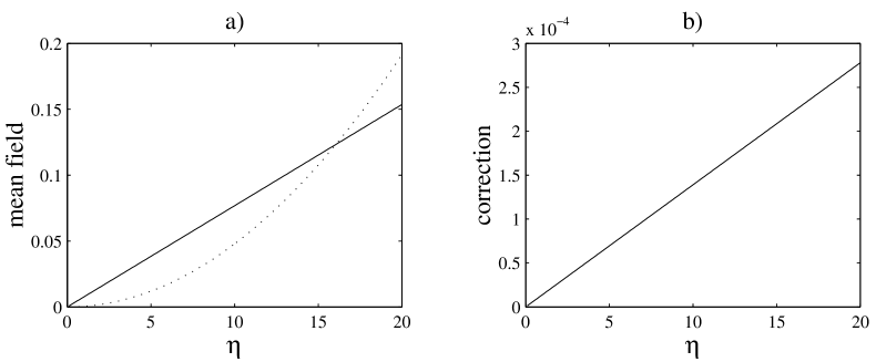
FIG. 6.: Boson-boson (solid line) and boson-fermion (dotted line) mean field contributions (a) and second-order corrections (b) to the ground-state energy-density of a ⁶Li, ⁷Li mixture, in units of $\epsilon_{\mbox{F}}$, to the ground-state energy-density in units of $\epsilon_{\mbox{F}}$. Parameters are $n_{\mbox{F}}^{1/3}a_{\mbox{BF}}=0.001$ and $n_{\mbox{B}}^{1/3}a_{\mbox{BB}}=0.000135\eta^{1/3}$, where the density ratio $\eta$ is the running independent variable.

In Fig. 6 we compare the mean field contributions (a) and second-order correction (b) to the energy functional for a ⁶Li, ⁷Li mixture, for a range of values of $\eta$. The plots correspond to a situation where the scattering lengths $a_{\mbox{BB}}=0.2$nm, $a_{\mbox{BF}}=2.7$nm and the fermion density $n_{\mbox{F}}=5.1\times 10^{10}$cm^-3 are fixed, and compatible with the experiments described in Ref. [14], while the boson density is varied. Note that for any reasonable boson density, the boson gas parameter $\beta$ is indeed very small compared to $\alpha$. In Fig. 7 we do the same for a ³He, ⁴He mixture. In this case the inter-species scattering length is unknown, however we conjecture it to be of the same order of magnitude as the boson-boson scattering length. The plots correspond to a situation where $a_{\mbox{BB}}=a_{\mbox{BF}}=16$nm, and $n_{\mbox{F}}=3.1\times 10^{13}$cm^-3. These values are compatible with current experiments on metastable triplet ⁴He condensates [18, 19], and are particularly interesting in that the beyond mean-field corrections are quite large (of the order of 10%). The true significance of the boson-fermion interaction energy correction will of course depend on the actual value of the interspecies scattering length. We notice that if the latter will turn out to be of about one order of magnitude larger than in the pure fermionic and bosonic cases (this is for instance what happens for lithium mixtures), then the effect of the correction can be as large as $50$% of the mean-field prediction. Then, of course, also corrections proportional to the boson gas parameter have to be taken into account.

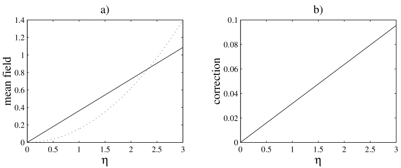
FIG. 7.: Boson-boson (solid line) and boson-fermion (dotted line) mean field contributions (a) and second-order corrections (b) to the ground-state energy-density of a ³He, ⁴He mixture, in units of $\epsilon_{\mbox{F}}$, to the ground-state energy-density in units of $\epsilon_{\mbox{F}}$. Parameters are $n_{\mbox{F}}^{1/3}a_{\mbox{BF}}=0.05$ and $n_{\mbox{B}}^{1/3}a_{\mbox{BB}}=0.05\eta^{1/3}$, where the density ratio $\eta$ is the running independent variable.

C Other physical quantities, Bose condensate depletion, and induced fermion-fermion interaction

From Eq. (103) we can readily determine the chemical potential for the fermions $\mu_{\mbox{F}}$, defined as

$$\mu_{\mbox{F}}=\left(\frac{\partial E/V}{\partial n_{\mbox{F}}}\right)_{N_{\mbox{B}},V},$$ (108)

to be

$$\mu_{\mbox{F}} = \frac{\hbar^{2}k_{\mbox{F}}^{2}}{2m_{\mbox{F}}}+\frac{2\pi\hbar^{2}a_{\mbox{BF}}}{m}n_{\mbox{B}}\left[1+\frac{4a_{\mbox{BF}}k_{\mbox{F}}}{3\pi}f(\delta)\right].$$ (109)

The pressure reads

$$P = -\left(\frac{\partial E}{\partial V}\right)_{N_{\mbox{B}},N_{\mbox{F}}}$$ (110)

$$= \frac{2}{5}\frac{\hbar^{2}k_{\mbox{F}}^{2}}{2m_{\mbox{F}}}n_{\mbox{F}}+\frac{2\pi n_{\mbox{B}}^{2}a_{\mbox{BB}}\hbar^{2}}{m_{\mbox{B}}}+\frac{2\pi\hbar^{2}a_{\mbox{BF}}}{m}n_{\mbox{F}}n_{\mbox{B}}\left[1+\frac{4a_{\mbox{BF}}k_{\mbox{F}}}{3\pi}f(\delta)\right].$$ (112)

We then obtain for the bosonic and fermionic compressibilities, respectively, for the bosons:

$$c_{\mbox{B}}^{2}=\frac{1}{m_{\mbox{B}}}\left(\frac{\partial P}{\partial n_{\mbox{B}}}\right)_{N_{\mbox{F}},V}$$ (113)

(114)

$$=\frac{4\pi n_{\mbox{B}}^{2}a_{\mbox{BB}}\hbar^{2}}{m^{2}_{\mbox{B}}}+\frac{2\pi\hbar^{2}a_{\mbox{BF}}}{m_{\mbox{B}}m}n_{\mbox{F}}\left[1+\frac{4a_{\mbox{BF}}k_{\mbox{F}}}{3\pi}f(\delta)\right],$$ (115)

and for the fermions:

$$c_{\mbox{F}}^{2} = \frac{1}{m_{\mbox{F}}}\left(\frac{\partial P}{\partial n_{\mbox{F}}}\right)_{N_{\mbox{B}},V}$$ (116)

$$= \frac{2}{3}\frac{\hbar^{2}k_{\mbox{F}}^{2}}{2m^{2}_{\mbox{F}}}+\frac{2\pi\hbar^{2}a_{\mbox{BF}}}{m_{\mbox{F}}m}n_{\mbox{B}}\left[1+\frac{16a_{\mbox{BF}}k_{\mbox{F}}}{9\pi}f(\delta)\right].$$ (118)

We notice that the possible instabilities induced by the mean-field boson-fermion interaction term in the case of a negative value of $a_{\mbox{BF}}$ are contrasted by the beyond mean-field correction, since the latter is always positive.

Concerning the structure of the Bose condensate fraction, besides the known depletion due to the boson-boson interaction, we expect in principle a further contribution to depletion due to the interaction of the bosons with the fermions. The depletion is computed in a standard way by integrating the boson propagator for the non condensed particles $G_{\mbox{B}}^{\prime}(p^{\mu})$ over four-momentum. To obtain the boson propagator we have to solve the Dyson equation (68) for $G_{\mbox{B}}^{\prime}(p^{\mu})$. This yields:

$$G_{\mbox{B}}^{\prime}(p^{\mu}) = \left[p^{0}+\frac{\hbar p^{2}}{2m_{\mbox{B}}}+\Sigma_{\mbox{B}}(-p^{\mu})-\Sigma_{\mbox{B}}(0)+\Sigma_{12}(0)\right]$$ (121)

$$\times\left\{\left[p^{0}-\frac{\Sigma_{\mbox{B}}(p^{\mu})-\Sigma_{\mbox{B}}(-p^{\mu})}{2}\right]^{2}\right.$$

$$\left.-\left[\frac{\hbar p^{2}}{2m_{\mbox{B}}}-\Sigma_{\mbox{B}}(0)+\Sigma_{12}(0)+\frac{\Sigma_{\mbox{B}}(p^{\mu})+\Sigma_{\mbox{B}}(-p^{\mu})}{2}\right]^{2}+\Sigma_{12}^{2}(p^{\mu})\right\}^{-1},$$

where we have made use of the Hugenholtz-Pines relation. The total diagonal bosonic self-energy $\Sigma_{\mbox{B}}(p^{\mu})$ picks up a boson-boson and a boson-fermion contribution (see Eq. (70)). It can be easily checked that to first order in $a_{\mbox{BB}}$ and in $a_{\mbox{BF}}$ the total diagonal bosonic self-energy does not depend on the four-momentum. Therefore the diagonal self-energy terms in the boson propagator Eq. (121) cancel, $G_{\mbox{B}}^{\prime}(p^{\mu})$ is independent of $a_{\mbox{BF}}$, and there is no depletion of the Bose condensate due to the fermions to this order, since the contribution of the fermions to the off-diagonal self-energies vanishes anyway in ladder approximation. The situation will be different to next order in $a_{\mbox{BF}}$, as in this case the total diagonal bosonic self-energy will depend on the four-momentum. However, the calculation of $\Sigma_{\mbox{B}}(p^{\mu})$ to second order in the boson-fermion scattering length at non zero four-momentum involves the evaluation of integrals that cannot be carried out analytically in a straightforward way. In conclusion, in the present situation, we will consider the depletion due to the bosons only, which is well known [25, 24]:

$$n_{\mbox{B}}-n_{0}=\frac{8}{3}\sqrt{\frac{n_{\mbox{B}}a_{\mbox{B}}^{3}}{\pi}}n_{\mbox{B}}\,.$$ (122)

We now turn to the discussion of the fermion-fermion interaction induced by the presence of the bosons. Subtracting the bosonic contribution from the energy density, we get

$$\frac{E}{V}-\epsilon_{\mbox{B}}=\epsilon_{\mbox{F}}\left[1+\frac{20\eta}{3\pi(1+\delta)}\alpha+\right.\left.\frac{20\eta}{3\pi(1+\delta)}\frac{f(\delta)}{\pi}\alpha^{2}\right].$$ (123)

This describes the first three terms of a power expansion in $\alpha$, of exactly the same form as that of an imperfect (unpolarized) Fermi gas, though clearly with different coefficients. There is thus, as expected, an induced fermion-fermion interaction, which can now be computed by exploiting the expressions that we have derived for both the bosonic and the fermionic chemical potentials. This will yield a modification of the known induced fermion-fermion interaction previously discussed in mean field approximation [17]. The expression for the induced interaction at zero energy-momentum transfer $U_{\mbox{ind}}(q^{\mu}=0)$ is :

$$U_{\mbox{ind}}(q^{\mu}=0)=\left.\frac{\partial\mu_{\mbox{F}}}{\partial n_{\mbox{F}}}\right|_{\mu_{\mbox{B}}}-\frac{\partial\mu_{\mbox{F}}}{\partial n_{\mbox{F}}}=-\left(\frac{\partial\mu_{\mbox{F}}}{\partial n_{\mbox{B}}}\right)^{2}\frac{\partial n_{\mbox{B}}}{\partial\mu_{\mbox{B}}}\,,$$ (124)

which in our case reads:

$$U_{\mbox{ind}}(q^{\mu}=0)=-\frac{4\pi\hbar^{2}(1-\delta^{2})\eta^{1/3}\alpha^{2}}{m_{\mbox{F}}k_{\mbox{F}}(6\pi^{2})^{1/3}\beta^{2/3}}\left[1+4f(\delta)\alpha/3\pi\right].$$ (125)

The extension to finite momentum transfer is achieved by introducing the boson density-density response function $\chi(q^{\mu})$, and is represented diagrammatically in Fig. 8, where two fermions interact by exchanging a boson density fluctuation wave. This is the simplest diagram by which two fermions can interact via the exchange of a bosonic excitation.

FIG. 8.: Effective fermion-fermion interaction due to exchange of boson density fluctuations.

The density-density response function $\chi(q^{\mu})$ is independent of $a_{\mbox{BF}}$ to first order. This can be easily verified following the same line of reasoning described previously in the analysis of the bosonic propagator. Thus its expression is the same as in the pure bosonic case (to this order):

$$\chi(q^{\mu})=\frac{\hbar n_{0}q^{2}/m_{\mbox{B}}}{(q^{0})^{2}-(\hbar q^{2}/2m_{\mbox{B}})^{2}-4\pi\hbar^{3}n_{0}a_{\mbox{BB}}q^{2}/m_{\mbox{B}}^{2}}\,.$$ (126)

The vertex $g_{\mbox{FF}}$ can be determined by considering the limiting expression for $\chi(q^{\mu})$ as $q^{\mu}\rightarrow 0$. In this case the expression for the diagram given in Fig. 8 must reduce to the expression given in Eq. (125). It follows that:

$$g_{\mbox{FF}}=\frac{2\sqrt{\pi}\hbar^{2}a_{\mbox{BF}}}{m}\left[1+4f(\delta)a_{\mbox{BF}}k_{\mbox{F}}/3\pi\right].$$ (127)

Then the induced interaction potential in the static case ($q^{0}=0$) reads:

$$U_{\mbox{ind}}(0,{\vec{q}})=-\frac{4\pi\hbar^{4}a^{2}_{\mbox{BF}}\left(1+4f(\delta)a_{\mbox{BF}}k_{\mbox{F}}/3\pi\right)^{2}}{m^{2}}\frac{n_{0}}{\hbar q^{2}/4m_{\mbox{B}}+4\pi\hbar^{2}n_{0}a_{\mbox{BB}}/m_{\mbox{B}}}\,.$$ (128)

In real space this is:

$$U_{\mbox{ind}}(0,{\vec{q}})=\frac{4\hbar^{2}m_{\mbox{B}}n_{0}a^{2}_{\mbox{BF}}\left(1+4f(\delta)a_{\mbox{BF}}k_{\mbox{F}}/3\pi\right)^{2}}{m^{2}}\frac{e^{\sqrt{2}r/\xi}}{r}\,,$$ (129)

where

$$\xi^{2}=\frac{1}{8\pi n_{0}a_{\mbox{B}}}\,.$$ (130)

We observe that, compared to the mean-field result [17], while there are quantitative modifications in the pre-factors, there is no qualitative change in the form of the induced interaction, i.e. we still have an attractive Yukawa potential. Modifications in the analytic form of the induced fermion-fermion interaction potential will appear only once second-order effects in the boson-fermion scattering length $a_{\mbox{BF}}$ to the depletion of the Bose condensate are included.

VI Discussion and Outlook

In summary, we have determined ground-state properties of a homogeneous system of bosons mixed with spin-polarized fermions at zero temperature. We have calculated the boson-fermion $T$-matrix and the corresponding self-energies. Then we have shown how to incorporate the effects of the boson-boson interaction and derived some relevant physical quantities of the system, in particular the ground-state energy. The importance of the beyond mean-field corrections has been discussed in several different instances of experimental interest. For mixtures of bosonic and fermionic Helium we have shown that the beyond mean-field terms may yield significant corrections (up to $50$% of the mean-field result). We have provided partial results also on two very significant physical quantities, namely the Bose condensate fraction and the induced fermion-fermion interaction. To provide more quantitative predictions for these quantities, as well as for the BCS transition temperature, we will need to compute in detail the corrections to second order in the boson-fermion scattering length. Results of this analysis, which goes beyond the scope of the present paper, will appear in a forthcoming work, together with a detailed numerical analysis of the conditions for stability and for phase separation. Collective modes, effective fermion mass, and excitation spectra fully evaluated to second order in the boson-fermion scattering length will be discussed as well.

Extensions of the formalism developed in this paper can be made in different directions. First, one can consider unpolarized spin-$1/2$ fermions. Calculations are very similar to the present situation with the main difference that one has to include the effects of the direct interactions of fermions with different spins. This would correspond to having a third scattering length $a_{\mbox{FF}}$. As in the previous case, we expect that in the two-particle scattering approximation the energy contribution for a pure fermion system of spin-$1/2$ fermions is simply added to Eq. (103) in this case (and of course, the Fermi momentum has to be modified appropriately).

The formalism can be also extended to consider finite temperature. As in the case of pure bosons we expect considerable difficulties near the critical temperature. Well below that temperature, however, we expect no major complications and the calculations will be similar to the present case, except that boson loops will have to be taken into account and frequency integrals will have to be replaced by Matsubara frequency sums.

A very important and natural possible extension is the investigation of inhomogeneous, e.g. harmonically trapped, systems. This can be done by augmenting the existing mean field calculations via the correlations terms in local density approximation. To this end, the results obtained in the present work are needed. The method and the full numerical procedure will be described in a forthcoming paper.

Finally, higher-order corrections may be in principle computed. These higher-order terms will involve also the bosonic gas parameter as well as three-particle correlations, and thus expansions like Eq. (103) will not reduce to sums of terms, where only one scattering length appears at a time, but will include also terms which contain products of powers of both scattering lengths. To even higher orders non-universal properties like the parameters describing the shape of the interaction potentials will become important and will have to be taken properly into account, as it has been recently done in the pure bosonic case [31, 45].

A Normal ordered products and the vacuum state

If we expand the field operators in terms of momentum eigenstates we get:

$$\hat{\Phi}({\mathbf{x}}) = \frac{1}{\sqrt{V}}\sum_{{\mathbf{k}}}\hat{a}_{{\mathbf{k}}}e^{i{\mathbf{k}}\cdot{\mathbf{x}}}=\frac{1}{\sqrt{V}}\hat{a}_{0}+\hat{\phi}({\mathbf{x}}),$$ (A1)

$$\hat{\Psi}({\mathbf{x}}) = \frac{1}{\sqrt{V}}\sum_{{\mathbf{k}}}\hat{b}_{{\mathbf{k}}}e^{i{\mathbf{k}}\cdot{\mathbf{x}}}=\hat{\psi_{1}}^{\dagger}({\mathbf{x}})+\hat{\psi_{2}}({\mathbf{x}}),$$ (A2)

with

$$\hat{\phi}({\mathbf{x}}) = \frac{1}{\sqrt{V}}\sum_{|{\mathbf{k}}|>0}\hat{a}_{{\mathbf{k}}}e^{i{\mathbf{k}}\cdot{\mathbf{x}}},$$ (A3)

$$\hat{\psi_{1}}({\mathbf{x}}) = \frac{1}{\sqrt{V}}\sum_{|{\mathbf{k}}|\leq k_{\mbox{F}}}\hat{b}^{\dagger}_{{\mathbf{k}}}e^{-i{\mathbf{k}}\cdot{\mathbf{x}}}\;,$$ (A4)

$$\hat{\psi_{2}}({\mathbf{x}}) = \frac{1}{\sqrt{V}}\sum_{|{\mathbf{k}}|>k_{\mbox{F}}}\hat{b}_{{\mathbf{k}}}e^{i{\mathbf{k}}\cdot{\mathbf{x}}}\;.$$ (A5)

In terms of the bosonic and fermionic occupation number operators $\hat{N}_{\mbox{B}}({\mathbf{k}})=\hat{a}^{\dagger}_{{\mathbf{k}}}\hat{a}_{{\mathbf{k}}}$ and $\hat{N}_{\mbox{F}}({\mathbf{k}})=\hat{b}^{\dagger}_{{\mathbf{k}}}\hat{b}_{{\mathbf{k}}}$ the ground state of the non-interacting system $|\xi_{0}\rangle$ can be characterized by:

$$\hat{N}_{\mbox{B}}(\vec{0})|\xi_{0}\rangle = N_{\mbox{B}}|\xi_{0}\rangle,$$ (A6)

$$\hat{N}_{\mbox{B}}({\mathbf{k}})|\xi_{0}\rangle = 0\mbox{ for }|{\mathbf{k}}|>0,$$ (A7)

$$\hat{N}_{\mbox{F}}({\mathbf{k}})|\xi_{0}\rangle = |\xi_{0}\rangle\mbox{ for }|{\mathbf{k}}|\leq k_{\mbox{F}},$$ (A8)

$$\hat{N}_{\mbox{F}}({\mathbf{k}})|\xi_{0}\rangle = 0\mbox{for}|{\mathbf{k}}|>k_{\mbox{F}}\,,$$ (A9)

where $N_{\mbox{B}}$ is the total number of bosons, which in this case coincides with the number of zero-momentum bosons $N_{0}$ (Bose-Einstein condensate). In occupation number representation we thus have

$$|\xi_{0}\rangle=|N_{\mbox{B}},0,0,\dots>_{\mbox{|B}}\otimes|1,1,\ldots,1,1,0,0,\ldots>_{\mbox{F}}\;,$$ (A10)

where the subscript B refers to the boson Hilbert space and the F to the fermion Hilbert space. The change from $1$ to $0$ in the fermion state happens at $k_{\mbox{F}}$. Additionally,

$$\hat{\phi}({\mathbf{x}})|\xi_{0}\rangle=\hat{\psi_{1}}({\mathbf{x}})|\xi_{0}\rangle=\hat{\psi_{2}}({\mathbf{x}})|\xi_{0}\rangle=0.$$ (A11)

In this sense the ground state can be regarded as the vacuum state with respect to fermions excited above the Fermi sea, the fermion holes below the Fermi sea, and the non-condensate bosons.

The normal product is defined on pairs of creation and destruction operators:

$$:\tilde{\phi}({\mathbf{x}},t)\tilde{\phi}^{\dagger}({\mathbf{x}}^{\prime},t^{\prime}): = \tilde{\phi}^{\dagger}({\mathbf{x}}^{\prime},t^{\prime})\tilde{\phi}({\mathbf{x}},t),$$ (A12)

$$:\tilde{\psi}_{j}({\mathbf{x}},t)\tilde{\psi}_{k}^{\dagger}({\mathbf{x}}^{\prime},t^{\prime}): = -\tilde{\psi}_{k}^{\dagger}({\mathbf{x}}^{\prime},t^{\prime})\tilde{\psi}_{j}({\mathbf{x}},t),$$ (A13)

$$:\tilde{\phi}({\mathbf{x}},t)\tilde{\psi}_{j}^{\dagger}({\mathbf{x}}^{\prime},t^{\prime}): = \tilde{\psi}_{j}^{\dagger}({\mathbf{x}}^{\prime},t^{\prime})\tilde{\phi}({\mathbf{x}},t),$$ (A14)

$$:\tilde{\psi}_{j}({\mathbf{x}},t)\tilde{\phi}^{\dagger}({\mathbf{x}}^{\prime},t^{\prime}): = \tilde{\phi}^{\dagger}({\mathbf{x}}^{\prime},t^{\prime})\tilde{\psi}_{j}({\mathbf{x}},t),$$ (A15)

for $j,k\in\{1,2\}$. For all other pairs of creation and destruction operators the normal product is the same as the ordinary operator product. It can also be readily determined that

$$[\tilde{\phi}({\mathbf{x}},t),\tilde{\phi}^{\dagger}(\vec{x^{\prime}},t^{\prime})] = \langle\xi_{0}|\tilde{\phi}({\mathbf{x}},t)\tilde{\phi}^{\dagger}({\mathbf{x}}^{\prime},t^{\prime})|\xi_{0}\rangle,$$ (A16)

$$\{\tilde{\psi}_{1}({\mathbf{x}}^{\prime},t^{\prime}),\tilde{\psi}^{\dagger}_{1}({\mathbf{x}},t)\} = \langle\xi_{0}|\tilde{\Psi}^{\dagger}({\mathbf{x}}^{\prime},t^{\prime})\tilde{\Psi}({\mathbf{x}},t)|\xi_{0}\rangle,$$ (A17)

$$\{\tilde{\psi}({\mathbf{x}},t),\tilde{\psi}^{\dagger}(\vec{x^{\prime}},t^{\prime})\} = \langle\xi_{0}|\tilde{\Psi}({\mathbf{x}},t)\tilde{\Psi}^{\dagger}({\mathbf{x}}^{\prime},t^{\prime})|\xi_{0}\rangle,$$ (A18)

and all other (anti-)commutators are zero. With Eqs. A15 and A18, the contractions of Eq. (37) can be readily evaluated.

B Evaluation of the $T$-Matrix and coupling constant renormalization

1 The first integral ${\cal I}$

We define

$${\cal I}=\int d^{3}{\mathbf{k}}\frac{\theta(|{\mathbf{P}}/2-{\mathbf{k}}|-k_{\mbox{F}})}{\hbar P^{0}-\hbar^{2}({\mathbf{P}}/2+{\mathbf{k}})^{2}/2m_{\mbox{B}}-\hbar^{2}({\mathbf{P}}/2-{\mathbf{k}})^{2}/2m_{\mbox{F}}+\mu+i\nu}.$$ (B1)

Transforming the integration variables to ${\mathbf{P}}/2-{\mathbf{k}}$ gives:

$${\cal I}=\int d^{3}{\mathbf{k}}\frac{\theta(|{\mathbf{k}}|-k_{\mbox{F}})}{\hbar^{2}{\mathbf{k}}^{2}/2m-\hbar^{2}{\mathbf{P}}\cdot{\mathbf{k}}/m_{\mbox{B}}-\hbar P^{0}+\hbar^{2}{\mathbf{P}}^{2}/2m_{\mbox{B}}-\mu-i\nu}.$$ (B2)

Setting $a=\hbar^{2}/2m$, $b=\hbar^{2}P/m_{\mbox{B}}$ and $E=-\hbar P^{0}+\hbar^{2}P^{2}/2m_{\mbox{B}}-\mu$ and transforming to spherical coordinates we get:

$${\cal I} = 2\pi\int^{k_{c}}_{k_{\mbox{F}}}dkk^{2}\int_{0}^{\pi}d\phi\sin\phi\frac{1}{ak^{2}-bk\cos\phi+E-i\nu}$$ (B3)

$$= \frac{2\pi}{b}\int^{k_{c}}_{k_{\mbox{F}}}dkk\ln\frac{ak^{2}-bk+E-i\nu}{ak^{2}+bk+E-i\nu},$$ (B4)

where we will ultimately consider the limit $k_{c}\to\infty$. Using $D=(b/2a)^{2}-E/a$ we can approximate for small $\nu$ (if $D\neq 0$; the case $D=0$ can be treated similarly and gives the same answer as taking the limit $D\to 0$ at the very end):

$${\cal I} = -\frac{2\pi m_{\mbox{B}}}{\hbar^{2}P}\int^{k_{c}}_{k_{\mbox{F}}}dkk$$ (B7)

$$\times\Biggl{(}\ln\frac{k+mP/m_{\mbox{B}}+\sqrt{D}+i\nu/2a\sqrt{D}}{k-mP/m_{\mbox{B}}-\sqrt{D}-i\nu/2a\sqrt{D}}$$

$$+\ln\frac{k+mP/m_{\mbox{B}}-\sqrt{D}-i\nu/2a\sqrt{D}}{k-mP/m_{\mbox{B}}+\sqrt{D}+i\nu/2a\sqrt{D}}\Biggr{)}.$$

The integral can be solved [44] to give

$$\lim_{k_{c}\to\infty}{\cal I} = -\frac{8\pi mk_{c}}{\hbar^{2}}+\frac{4\pi mk_{\mbox{F}}}{\hbar^{2}}$$ (B12)

$$+\frac{\pi}{\hbar^{2}}\left(\frac{m_{\mbox{B}}k_{\mbox{F}}^{2}}{P}-\frac{m^{2}P}{m_{\mbox{B}}}-2m\sqrt{D}-\frac{m_{\mbox{B}}D}{P}\right)$$

$$\times\ln\frac{k_{\mbox{F}}+mP/m_{\mbox{B}}+\sqrt{D}+i\nu/2a\sqrt{D}}{k_{\mbox{F}}-mP/m_{\mbox{B}}-\sqrt{D}-i\nu/2a\sqrt{D}}$$

$$-\frac{\pi}{\hbar^{2}}\left(\frac{m_{\mbox{B}}k_{\mbox{F}}^{2}}{P}-\frac{m^{2}P}{m_{\mbox{B}}}+2m\sqrt{D}-\frac{m_{\mbox{B}}D}{P}\right)$$

$$\times\ln\frac{k_{\mbox{F}}-mP/m_{\mbox{B}}+\sqrt{D}+i\nu/2a\sqrt{D}}{k_{\mbox{F}}+mP/m_{\mbox{B}}-\sqrt{D}-i\nu/2a\sqrt{D}},$$

where outside the logarithms we have taken the limit $\nu\to 0$ (simply setting $\nu=0$), and we have made use of the identity

$$\lim_{x\to\infty}x^{2}\ln\frac{1+\alpha/x}{1-\alpha/x}=2\alpha x,$$ (B13)

for the limit $k_{c}\to\infty$. There remains an ultraviolet divergent term; the boson-fermion $T$-matrix [Eq. (87)] is however ultimately renormalized by the second integral.

The real part of $\cal{I}$ is readily evaluated in the limit $\nu\to 0$ by setting $\nu=0$ and using the absolute values inside the logarithms:

$$\lim_{\nu\to 0}\mbox{Re}{\cal I} = -\frac{8\pi mk_{c}}{\hbar^{2}}+\frac{4\pi mk_{\mbox{F}}}{\hbar^{2}}$$ (B17)

$$+\frac{\pi}{\hbar^{2}}\left(\frac{m_{\mbox{B}}k_{\mbox{F}}^{2}}{P}-\frac{m^{2}P}{m_{\mbox{B}}}-\frac{m_{\mbox{B}}D}{P}\right)$$

$$\times\ln\left|\frac{(k_{\mbox{F}}+mP/m_{\mbox{B}})^{2}-D}{(k_{\mbox{F}}-mP/m_{\mbox{B}})^{2}-D}\right|$$

$$-\frac{2\pi m}{\hbar^{2}}\sqrt{D}\ln\left|\frac{(k_{\mbox{F}}+\sqrt{D})^{2}-(mP/m_{\mbox{B}})^{2}}{(k_{\mbox{F}}-\sqrt{D})^{2}-(mP/m_{\mbox{B}})^{2}}\right|.$$

Using the identity (easily evaluated by polar decomposition)

$$\lim_{\nu\to 0^{+}}\mbox{Im}\ln\frac{a+i\nu}{b-i\nu}=\left\{\begin{array}[]{r@{\quad:\quad}l}0&\mbox{sgn}(a)=\mbox{sgn}(b)\\ \pi&\mbox{sgn}(a)\neq\mbox{sgn}(b)\\ \end{array}\right.,$$ (B19)

the imaginary part of ${\cal I}$ in the limit $\nu\to 0$ can be evaluated to be:

$$\lim_{\nu\to 0}\mbox{Im}{\cal I}=\frac{\pi^{2}}{\hbar^{2}}\left(\frac{m_{\mbox{B}}k_{\mbox{F}}^{2}}{P}-\frac{m^{2}P}{m_{\mbox{B}}}-2m\sqrt{D}-\frac{m_{\mbox{B}}D}{P}\right),$$ (B20)

if $D>0$ and $k_{\mbox{F}}<|mP/m_{\mbox{B}}-\sqrt{D}|$;

$$\lim_{\nu\to 0}\mbox{Im}{\cal I}=-\frac{4\pi^{2}m\sqrt{D}}{\hbar^{2}},$$ (B21)

if $D>0$ and $|mP/m_{\mbox{B}}-\sqrt{D}|<k_{\mbox{F}}<mP/m_{\mbox{B}}+\sqrt{D}$; and

$$\lim_{\nu\to 0}\mbox{Im}{\cal I}=0,$$ (B22)

if $D\leq 0$ or $k_{\mbox{F}}>mP/m_{\mbox{B}}+\sqrt{D}$.

2 The second integral ${\cal J}$

We define

$${\cal J} = -\int d^{3}{\mathbf{k}}\frac{1}{\hbar^{2}{\mathbf{k}}_{1}^{2}/2m-\hbar^{2}{\mathbf{k}}^{2}/2m+i\nu}$$ (B23)

$$= \frac{4\pi}{a}\int_{0}^{k_{c}}dk\left(1-\frac{k_{1}^{2}+i\nu/a}{k^{2}-k_{1}^{2}-i\nu/a}\right),$$ (B24)

where as before $a=\hbar^{2}/2m$, and we have transformed to polar coordinates and integrated over the angle variables. The integral can be evaluated [44] to give

$${\cal J} = \frac{4\pi k_{c}}{a}-\frac{2\pi}{a}\sqrt{k_{1}^{2}-i\nu/a}\ln\frac{k_{c}+\sqrt{k_{1}^{2}-i\nu/a}}{k_{c}-\sqrt{k_{1}^{2}-i\nu/a}}$$ (B26)

$$+\frac{2\pi}{a}\sqrt{k_{1}^{2}-i\nu/a}\ln\frac{\sqrt{k_{1}^{2}-i\nu/a}}{-\sqrt{k_{1}^{2}-i\nu/a}}.$$

We then use

$$\lim_{k_{c}\to\infty}\ln\frac{k_{c}+\sqrt{k_{1}^{2}-i\nu/a}}{k_{c}-\sqrt{k_{1}^{2}-i\nu/a}}=0$$ (B27)

to get

$$\lim_{\nu\to 0}{\cal J} = \frac{8\pi mk_{c}}{\hbar^{2}}+i\frac{4\pi^{2}mk_{1}}{\hbar^{2}}.$$ (B28)

If we now take the sum of Eqs. (B12) and (B28), the ultraviolet divergent terms cancel exactly. The resulting expression for ${\cal I}+{\cal J}$ can then be substituted into Eq. (87) to get Eq. (92) for the renormalized boson-fermion $T$-matrix.

REFERENCES

- [1] M. H. Anderson, J. R. Ensher, M. R. Matthews, C. E. Wieman, and E. A. Cornell, Science 269, 198 (1995).
- [2] K. B. Davis, M.-O. Mewes, M. R. Andrews, N. J. van Druten, D. S. Durfee, D. M. Kurn, and W. Ketterle, Phys. Rev. Lett. 75, 3969 (1995).
- [3] C. C. Bradley, C. A. Sackett, J. J. Tollett, and R. Hulet, Phys. Rev. Lett. 75, 1687 (1995).
- [4] F. Dalfovo, S. Giorgini, L. P. Pitaevskii, and S. Stringari, Rev. Mod. Phys. 71, 463 (1999).
- [5] Bose-Einstein Condensation in Atomic Gases, edited by M. Inguscio, S. Stringari, and C. Wieman (IOS Press, Amsterdam 1999).
- [6] W. Ketterle, Phys. Today 52 (12), 30 (1999).
- [7] A. J. Leggett, Rev. Mod. Phys. 73, 307 (2001).
- [8] G. Baym, J. Phys. B 34, 4541 (2001).
- [9] B. DeMarco and D. S. Jin, Science 285, 1703 (1999).
- [10] B. DeMarco, S. B. Papp, and D. S. Jin, Phys. Rev. Lett. 86, 5409 (2001).
- [11] J. Goldwin, S. B. Papp, B. DeMarco, and D. S. Jin, e-print cond-mat/0108287.
- [12] A. G. Truscott, K. E. Strecker, W. I. McAlexander, G. B. Partridge, and R. G. Hulet, Science 291, 2570 (2001).
- [13] F. Schreck, G. Ferrari, K. L. Corwin, J. Cubizolles, L. Khaykovich, M.-O. Mewes, and C. Salomon, Phys. Rev. A 64, 011402(R) (2001).
- [14] F. Schreck, L. Khaykovich, K. L. Corwin, G. Ferrari, T. Bourdel, J. Cubizolles, and C. Salomon, Phys. Rev. Lett. 87, 080403 (2001).
- [15] H. T. C. Stoof, M. Houbiers, C. A. Sackett, and R. G. Hulet, Phys. Rev. Lett. 76, 10 (1996).
- [16] M. Holland, S. J. J. M. F. Kokkelmans, M. L. Chiofalo, and R. Walser, Phys. Rev. Lett. 87, 120406 (2001).
- [17] L. Viverit, C. J. Pethick, and H. Smith, Phys. Rev. A 61, 053605 (2000).
- [18] A. Robert, O. Sirjean, A. Browaeys, J. Poupard, S. Nowak, D. Boiron, C. I. Westbrook, A. Aspect, Science 292, 461 (2001).
- [19] F. Pereira Dos Santos, J. Léonard, J. Wang, C. J. Barralet, F. Perales, E. Rasel, C. S. Unnikrishnan, M. Leduc, and C. Cohen-Tannoudji, Phys. Rev. Lett. 86, 3459 (2001).
- [20] N. Nygaard and K. Mølmer, Phys. Rev. A 59, 2974 (1999).
- [21] M. J. Bijlsma, B. A. Heringa, and H. T. C. Stoof, Phys. Rev. A 61, 053601 (2000).
- [22] H. Pu, W Zhang, M. Wilkens, and P. Meystre e-print: cond-mat/0104279.
- [23] V. Galittskii, Sov. Phys. JETP 7, 104 (1958).
- [24] A. A. Abrikosov, L. P. Gorkov, and I. E. Dzyaloshinski, Methods of Quantum Field Theory in Statistical Physics, (Dover Publications, New York, 1963).
- [25] A. L. Fetter and J. D. Walecka, Quantum Theory of Many-Particle Systems, (McGraw-Hill, New York, 1971).
- [26] T. T. Lee and C. N. Yang Phys. Rev. 105, 1119 (1957).
- [27] S. Beliaev, Sov. Phys. JETP 7, 299 (1958).
- [28] N. Hugenholtz and D. Pines, Phys. Rev. A 99, 489 (1959).
- [29] T. T. Wu, Phys. Rev. 115, 1390 (1959).
- [30] K. Sawada, Phys. Rev. 116, 1344 (1959).
- [31] E. Braaten and A. Nieto, Eur. Phys. J. B 11, 143 (1999).
- [32] W. F. Saam, Ann. Phys. 53, 239 (1969).
- [33] A. Galindo and P. Pascual Quantum Mechanics Vol. II, (Springer-Verlag, Berlin, 1990).
- [34] This is only true for spin-polarized fermions. In general , where is the spin-degeneracy.
- [35] N. Bogoliubov, J. Phys. (USSR) 11, 23 (1947).
- [36] M. Girardeau and R. Arnowitt, Phys. Rev. 113, 755 (1959).
- [37] C. W. Gardiner, Phys. Rev. A 56, 1414 (1997).
- [38] Y. Castin and R. Dum, Phys. Rev. A 57, 3008 (1998).
- [39] S. A. Morgan, J. Phys. B 33, 3847 (2000).
- [40] G. C. Wick, Phys. Rev. 80, 268 (1950).
- [41] Considering Eq. (7.12) of Ref. [25], we take , and replace by and by . The derivation is then the same, apart from some sign factors.
- [42] The proof of the validity of the Hugenholtz-Pines theorem can be adopted litteraly from the pure boson case, since it is based on how to replace condensate lines by non-condensate propagators; a procedure, which is unchanged in the present situation.
- [43] This could possibly be realized by a Feschbach resonance, with the effective boson-boson scattering length tuned down to nearly zero. See: J. Stenger, S. Inouye, M. R. Andrews, H.-J. Miesner, D. M. Stamper-Kurn, and W. Ketterle, Phys. Rev. Lett. 82, 2422 (1999); S. L. Cornish, N. R. Claussen, J. L. Roberts, E. A. Cornell, and C. E. Wieman, Phys. Rev. Lett. 85, 1795 (2000).
- [44] A. P. Prudnikov, Yu. A. Brychkov, and O. I. Marichev, Integrals and Series, Vol. 1, (Gordon and Breach Science Publishers, Amsterdam ,1998).
- [45] E. Braaten, W. H. Hammer, and S. Hermans, Phys. Rev. A 63, 063609 (2001).