Many-body Green’s function theory for thin ferromagnetic films: exact treatment of the single-ion anisotropy

P. Fröbrich⁺, P.J. Kuntz, and M. Saber⁺⁺

Hahn-Meitner-Institut Berlin, Glienicker Straße 100, D-14109 Berlin, Germany,
⁺also: Institut für Theoretische Physik, Freie Universität Berlin
Arnimallee 14, D-14195 Berlin, Germany
⁺⁺ home address: Physics Department, Faculty of Sciences, University Moulay Ismail, B.P. 4010 Meknes, Morocco

Abstract. A theory for the magnetization of ferromagnetic films is formulated within the framework of many-body Green’s function theory which considers all components of the magnetization. The model Hamiltonian includes a Heisenberg term, an external magnetic field, a second- and fourth-order uniaxial single-ion anisotropy, and the magnetic dipole-dipole coupling. The single-ion anisotropy terms can be treated exactly by introducing higher-order Green’s functions and subsequently taking advantage of relations between products of spin operators which leads to an automatic closure of the hierarchy of the equations of motion for the Green’s functions with respect to the anisotropy terms. This is an improvement on the method of our previous work, which treated the corresponding terms only approximately by decoupling them at the level of the lowest-order Green’s functions. RPA-like approximations are used to decouple the exchange interaction terms in both the low-order and higher-order Green’s functions. As a first numerical example we apply the theory to a monolayer for spin $S=1$ in order to demonstrate the superiority of the present treatment of the anisotropy terms over the previous approximate decouplings.

Keywords: Quantized spin model; Many-body Green’s functions; thin ferromagnetic films.

1 Introduction

There is increasing activity in experimental and theoretical investigations of the properties of thin magnetic films and multi-layers. Of particular interest is the magnetic reorientation transition which is measured as function of temperature and film thickness; for recent papers, see [1, 2] and references therein.

The simplest theoretical approach to the treatment of thin ferromagnetic films in the Heisenberg model is the mean field theory (MFT), which can be applied either by diagonalization of a single-particle Hamiltonian[3] or by thermodynamic perturbation theory[4]. This approximation, however, completely neglects collective excitations (spin waves), which are known to be much more important for the magnetic properties of 2D systems than for 3D bulk materials. In order to take the influence of collective excitations into account, one can turn to many-body Green’s function theory (GFT), which allows reliable calculations over the entire range of temperature of interest: see, for example, Refs. [5, 6, 7], where the formalism includes the magnetic reorientation. The application of Green’s functions after a Holstein-Primakoff mapping to bosons, as applied in Ref. [8], is valid only at low temperatures. Another method, which also can treat the magnetic reorientation for all temperatures, is the application of a Schwinger-Boson theory[9]. Classical Monte Carlo calculations are also able to simulate the reorientation transition (see [10] and references therein). The temperature-dependent reorientation transition has also been investigated with a Hubbard model[11].

In the present paper, we apply a Green’s function theory to a Heisenberg Hamiltonian plus anisotropy terms, a system previously treated at the level of the lowest-order Green’s functions[5, 6, 7]. The approximate treatment of the single-ion anisotropy in the previous work is avoided here by extending the formalism to higher-order Green’s functions and applying relations for products of spin operators, a procedure which leads to automatic closure of the hierarchy of equations of motion with respect to those terms stemming from the single-ion anisotropy. The exchange terms occurring in the higher-order Green’s functions must, however, still be decoupled in an RPA-like fashion. This can be considered as an extension of the work of Devlin[12], who has applied higher-order Green’s functions to the description of bulk magnetic materials in one direction only. Our formulation applies to all spatial directions of a multi-layer system. We formulate the theory explicitly for a monolayer for spin $S=1$ and give equations for an extension to the multi-layer case. It is straightforward to see how the theory could be applied to higher spins.

The paper is organized as follows: in Section 2, the previous theory[5, 6] for thin ferromagnetic films is generalized by introducing higher-order Green’s functions, the model being explained in detail for a monolayer with $S=1$. Section 3 gives the formal extension to the multi-layer case. In Section 4, numerical results for the $S=1$ monolayer demonstrate the superiority of the exact treatment of the single-ion anisotropy term over the previously applied[5, 6] Anderson-Callen[13] decoupling. Section 5 contains a summary of the results.

2 The Green’s function formalism

We investigate here a spin Hamiltonian, nearly the same as in Ref. [6], consisting of an isotropic Heisenberg exchange interaction between nearest neighbour lattice sites, $J_{kl}$, second- and fourth-order single-ion lattice anisotropies with strengths $K_{2,k}$ and $K_{4,k}$ respectively, a magnetic dipole coupling with strength $g_{kl}$, and an external magnetic field ${\bf{B}}=(B^{x},B^{y},B^{z})$:

$${\cal H} = -\frac{1}{2}\sum_{<kl>}J_{kl}(S_{k}^{-}S_{l}^{+}+S_{k}^{z}S_{l}^{z})$$ (1)

$$-\sum_{k}K_{2,k}(S_{k}^{z})^{2}-\sum_{k}K_{4,k}(S_{k}^{z})^{4}$$

$$-\sum_{k}\Big{(}\frac{1}{2}B^{-}S_{k}^{+}+\frac{1}{2}B^{+}S_{k}^{-}+B^{z}S_{k}^{z}\Big{)}$$

$$+\frac{1}{2}\sum_{kl}\frac{g_{kl}}{r_{kl}^{5}}\Big{(}r_{kl}^{2}(S_{k}^{-}S_{l}^{+}+S_{k}^{z}S_{l}^{z})-3({\bf{S}}_{k}\cdot{\bf{r}}_{kl})({\bf{S}}_{l}\cdot{\bf r}_{kl})\Big{)}\ .$$

Here the notation $S_{i}^{\pm}=S_{i}^{x}\pm iS_{i}^{y}$ and $B^{\pm}=B^{x}\pm iB^{y}$ is introduced, where $k$ and $l$ are lattice site indices, and $\langle kl\rangle$ indicates summation over nearest neighbours only. Here, we add to the Hamiltonian in Ref. [6] a fourth-order anisotropy term which we can treat exactly but for which we previously had no decoupling procedure available.

Each layer is assumed to be ferromagnetically ordered: spins on each site in the same layer are parallel, whereas spins belonging to different layers need not be. Furthermore, the anisotropy strengths, coupling constants and magnetic moments are considered to be layer-dependent, so that inhomogeneous systems can be considered.

To allow as general a formulation as possible (with an eye to a future study of the reorientation of the magnetization), we formulate the equations of motion for the Green’s functions for all spatial directions:

$$G_{ij}^{+,\mp}(\omega) = \langle\langle S_{i}^{+};S_{j}^{\mp}\rangle\rangle_{\omega}$$

$$G_{ij}^{-,\mp}(\omega) = \langle\langle S_{i}^{-};S_{j}^{\mp}\rangle\rangle_{\omega}$$ (2)

$$G_{ij}^{z,\mp}(\omega) = \langle\langle S_{i}^{z};S_{j}^{\mp}\rangle\rangle_{\omega}\ .$$

Instead of decoupling the corresponding equations of motion at this stage, as we did in our previous work[5, 6], we add equations for the next higher-order Green’s functions:

$$G_{ij}^{z+,\mp}(\omega) = \langle\langle(2S_{i}^{z}-1)S_{i}^{+};S_{j}^{\mp}\rangle\rangle_{\omega}$$

$$G_{ij}^{-z,\mp}(\omega) = \langle\langle S_{i}^{-}(2S_{i}^{z}-1);S_{j}^{\mp}\rangle\rangle_{\omega}$$

$$G_{ij}^{++,\mp}(\omega) = \langle\langle S_{i}^{+}S_{i}^{+};S_{j}^{\mp}\rangle\rangle_{\omega}$$ (3)

$$G_{ij}^{--,\mp}(\omega) = \langle\langle S_{i}^{-}S_{i}^{-};S_{j}^{\mp}\rangle\rangle_{\omega}$$

$$G_{ij}^{zz,\mp}(\omega) = \langle\langle(6S_{i}^{z}S_{i}^{z}-2S(S+1));S_{j}^{\mp}\rangle\rangle_{\omega}\ .$$

The particular form for the operators used in the definition of the Green’s functions in Eqs. (2 The Green’s function formalism) is dictated by expressions coming from the anisotropy terms. Terminating the hierarchy of the equations of motion at this level of the Green’s functions results in an exact treatment of the anisotropy terms for spin $S=1$, since the hierarchy for these terms breaks off at this stage, as will be shown. The exchange interaction terms, however, still have to be decoupled, which we do with RPA-like decouplings.

For the treatment of arbitrary spin $S$, it is necessary to use $4S(S+1)$ Green’s functions in order to obtain an automatic break-off of the equations-of-motion hierarchy coming from the anisotropy terms. These are functions of the structure $G_{ij}^{\alpha,\mp}$ with $\alpha=(z)^{n}(+)^{m}$ and $\alpha=(-)^{m}(z)^{n}$, where, for a particular spin $S$, all combinations of $m$ and $n$ satisfying $(n+m)=2S$ have to be taken into account. There occur no Green’s functions having mixed $+$ and $-$ indices, because these can be reduced by the relation $S^{\mp}S^{\pm}=S(S+1)\mp S^{z}-(S^{z})^{2}$.

The equations of motion which determine the Green’s functions are

$$\omega G_{ij}^{\alpha,\mp}=A_{i,j}^{\alpha,\mp}+\langle\langle[O_{i}^{\alpha},{\cal H}]_{-};S_{j}^{\mp}\rangle\rangle,$$ (4)

with the inhomogeneities

$$A_{ij}^{\alpha,\mp}=\langle[O_{i}^{\alpha},S_{j}^{\mp}]_{-}\rangle,$$ (5)

where $O_{i}^{\alpha}$ are the operators occuring in the definition of the Green’s functions, and $\langle...\rangle=Tr(...e^{-\beta{\cal H}})$.

In the following, we treat a monolayer with $S=1$ explicitly. In this case, a system of 8 equations of motion is necessary:

$$\omega G_{ij}^{+,\mp} = A_{ij}^{+,\mp}-\sum_{k}J_{ik}\langle\langle S_{i}^{z}S_{k}^{+}-S_{k}^{z}S_{i}^{+};S_{j}^{\mp}\rangle\rangle+B^{z}G_{ij}^{+,\mp}-B^{+}G_{ij}^{z,\mp}$$

$$+(K_{2,i}+K_{4,i})G_{ij}^{z+,\mp}-2K_{i,4}(G_{ij}^{(z)^{2}+,\mp}-G_{ij}^{(z)^{3}+,\mp}),$$

$$\omega G_{ij}^{-,\mp} = A_{ij}^{-,\mp}+\sum_{k}J_{ik}\langle\langle S_{i}^{z}S_{k}^{-}-S_{k}^{z}S_{i}^{-};S_{j}^{\mp}\rangle\rangle-B^{z}G_{ij}^{-,\mp}+B^{-}G_{ij}^{z,\mp}$$

$$-(K_{2,i}+K_{4,i})G_{ij}^{-z,\mp}+2K_{i,4}(G_{ij}^{-(z)^{2},\mp}-G_{ij}^{-(z)^{3},\mp}),$$

$$\omega G_{ij}^{z,\mp} = A_{ij}^{z,\mp}+\frac{1}{2}\sum_{k}J_{ik}\langle\langle S_{i}^{-}S_{k}^{+}-S_{k}^{-}S_{i}^{+};S_{j}^{\mp}\rangle\rangle-\frac{1}{2}B^{-}G_{ij}^{+,\mp}+\frac{1}{2}B^{+}G_{ij}^{-,\mp},$$

$$\omega G_{ij}^{z+,\mp} = A_{ij}^{z+,\mp}-\frac{1}{2}\sum_{k}J_{ik}\Big{(}\langle\langle(6S_{i}^{z}S_{i}^{z}-2S(S+1))S_{k}^{+};S_{j}^{\mp}\rangle\rangle$$

$$+2\langle\langle S_{k}^{-}S_{i}^{+}S_{i}^{+};S_{j}^{\mp}\rangle\rangle-2\langle\langle S_{k}^{z}(S_{i}^{z}S_{i}^{+}+S_{i}^{+}S_{i}^{z});S_{j}^{\mp}\rangle\rangle\Big{)}$$

$$-B^{-}G_{ij}^{++,\mp}-\frac{1}{2}B^{+}G_{ij}^{zz,\mp}+B^{z}G_{ij}^{z+,\mp}$$

$$-(K_{2,i}+K_{4,i})G_{ij}^{z+,\mp}+(2K_{2,i}+4K_{4,i})G_{ij}^{(z)^{2}+,\mp}-6K_{i,4}G_{ij}^{(z)^{3}+,\mp}+4K_{4,i}G_{ij}^{(z)^{4}+,\mp},$$

$$\omega G_{ij}^{-z,\mp} = A_{ij}^{-z,\mp}+\frac{1}{2}\sum_{k}J_{ik}\Big{(}\langle\langle S_{k}^{-}(6S_{i}^{z}S_{i}^{z}-2S(S+1));S_{j}^{\mp}\rangle\rangle$$

$$+2\langle\langle S_{i}^{-}S_{i}^{-}S_{k}^{+};S_{j}^{\mp}\rangle\rangle-2\langle\langle S_{k}^{z}(S_{i}^{z}S_{i}^{-}+S_{i}^{-}S_{i}^{z});S_{j}^{\mp}\rangle\rangle\Big{)}$$

$$+\frac{1}{2}B^{-}G_{ij}^{zz,\mp}+B^{+}G_{ij}^{--,\mp}-B^{z}G_{ij}^{-z,\mp}$$

$$+(K_{2,i}+K_{4,i})G_{ij}^{-z,\mp}-(2K_{2,i}+4K_{4,i})G_{ij}^{-(z)^{2},\mp}+6K_{i,4}G_{ij}^{-(z)^{3},\mp}-4K_{4,i}G_{ij}^{-(z)^{4},\mp},$$

$$\omega G_{ij}^{++,\mp} = A_{ij}^{++,\mp}-\sum_{k}J_{ik}\Big{(}\langle\langle(S_{i}^{z}S_{i}^{+}+S_{i}^{+}S_{i}^{z})S_{k}^{+};S_{j}^{\mp}\rangle\rangle-2\langle\langle S_{i}^{+}S_{i}^{+}S_{k}^{z};S_{j}^{\mp}\rangle\rangle\Big{)}$$

$$-B^{+}G_{ij}^{z+,\mp}+2B^{z}G_{ij}^{++,\mp}-4K_{2,i}(G_{ij}^{++,\mp}-G_{ij}^{z++,\mp})$$

$$-K_{i,4}(8G_{ij}^{(z)^{3}++,\mp}-24G_{ij}^{(z)^{2}++,\mp}+32G_{ij}^{z++,\mp}-16G_{ij}^{++,\mp}),$$

$$\omega G_{ij}^{--,\mp} = A_{ij}^{--,\mp}+\sum_{k}J_{ik}\Big{(}\langle\langle S_{k}^{-}(S_{i}^{z}S_{i}^{-}+S_{i}^{-}S_{i}^{z});S_{j}^{\mp}\rangle\rangle-2\langle\langle S_{i}^{-}S_{i}^{-}S_{k}^{z};S_{j}^{\mp}\rangle\rangle\Big{)}$$

$$+B^{-}G_{ij}^{-z,\mp}-2B^{z}G_{ij}^{--,\mp}+4K_{2,i}(G_{ij}^{--,\mp}-G_{ij}^{--z,\mp})$$

$$-K_{i,4}(8G_{ij}^{--(z)^{3},\mp}-24G_{ij}^{--(z)^{2},\mp}+32G_{ij}^{--z,\mp}-16G_{ij}^{--,\mp}),$$

$$\omega G_{ij}^{zz,\mp} = A_{ij}^{zz,\mp}+\sum_{k}J_{ik}\Big{(}3\langle\langle(S_{i}^{z}S_{i}^{-}+S_{i}^{-}S_{i}^{z})S_{k}^{+};S_{j}^{\mp}\rangle\rangle-3\langle\langle S_{k}^{-}(S_{i}^{z}S_{i}^{+}+S_{i}^{+}S_{i}^{z});S_{j}^{\mp}\rangle\rangle\Big{)}$$ (6)

$$-3B^{-}G_{ij}^{z+,\mp}+3B^{+}G_{ij}^{-z,\mp}.$$

These equations are exact. The important point now is that the anisotropy terms in these equations can be simplified by using formulae which reduce products of spin operators by one order. Such relations were derived in Ref. [14]:

$$(S^{-})^{m}(S^{z})^{2S+1-m} = (S^{-})^{m}\sum_{i=0}^{2S-m}\delta_{i}^{(S,m)}(S^{z})^{i},$$

$$(S^{z})^{2S+1-m}(S^{+})^{m} = \sum_{i=0}^{2S-m}\delta_{i}^{(S,m)}(S^{z})^{i}(S^{+})^{m}.$$ (7)

The coefficients $\delta_{i}^{(S,m)}$ are tabulated in Ref. [14] for general spin. For spin $S=1$, only the coefficients with $m=0,1,2$ occur: $\delta_{0}^{(1,0)}=\delta_{2}^{(1,0)}=0;\delta_{1}^{(1,0)}=1,\delta_{0}^{(1,1)}=0,\delta_{1}^{(1,1)}=1,\delta_{0}^{(1,2)}=1$.

Application of these relations, effects the reduction of the relevant Green’s functions coming from the anisotropy terms in equations (2 The Green’s function formalism):

$$G_{ij}^{(z)^{4}+,\mp} = G_{ij}^{(z)^{3}+,\mp}=G_{ij}^{(z)^{2}+,\mp}=\frac{1}{2}(G_{ij}^{z+,\mp}+G_{ij}^{+,\mp}),$$

$$G_{ij}^{-(z)^{4},\mp} = G_{ij}^{-(z)^{3},\mp}=G_{ij}^{-(z)^{2},\mp}=\frac{1}{2}(G_{ij}^{-z,\mp}+G_{ij}^{-,\mp}),$$

$$G_{ij}^{(z)^{2}++,\mp} = G_{ij}^{z++,\mp}=G_{ij}^{++,\mp},$$ (8)

$$G_{ij}^{--(z)^{2},\mp} = G_{ij}^{--z,\mp}=G_{ij}^{--,\mp}.$$

The higher Green’s functions coming from the anisotropy terms have thus been expressed in terms of the lower-order functions already present in the hierarchy; i.e. with respect to the anisotropy terms, a closed system of equations of motion results, so that no decoupling of these terms is necessary. In other words, the anisotropy is treated exactly. For higher spins, $S>1$, one can proceed analogously. For this, one needs even higher-order Green’s functions but again, applying equations (2 The Green’s function formalism) reduces the relevant Green’s functions by one order, which in turn leads to a closed system of equations obviating the decoupling of terms coming from the anisotropies.

No such procedure is available for the exchange interaction terms, however, so that these still have to be decoupled. For spin $S=1$, we use RPA-like approximations to effect the decoupling:

$$\langle\langle S_{i}^{\alpha}S_{k}^{\beta};S_{j}^{\mp}\rangle\rangle \simeq \langle S_{i}^{\alpha}\rangle G_{kj}^{\beta,\mp}+\langle S_{k}^{\beta}\rangle G_{ij}^{\alpha,\mp}$$

$$\langle\langle S_{k}^{\alpha}S_{i}^{\beta}S_{i}^{\gamma};S_{j}^{\mp}\rangle\rangle \simeq \langle S_{k}^{\alpha}\rangle G_{ij}^{\beta\gamma,\mp}+\langle S_{i}^{\beta}S_{i}^{\gamma}\rangle G_{kj}^{\alpha,\mp}.$$ (9)

Note that we have constructed the decoupling so as not to break correlations having equal indices, since the corresponding operators form the algebra characterizing the group for a spin $S=1$ system. For spin $S=1$, this decoupling model leads to 8 diagonal correlations for each layer $i$:

$\langle S_{i}^{+}\rangle,\langle S_{i}^{-}\rangle,\langle S_{i}^{z}\rangle,$ $\langle S_{i}^{+}S_{i}^{+}\rangle,\langle S_{i}^{-}S_{i}^{-}\rangle,\langle S_{i}^{z}S_{i}^{z}\rangle,\langle S_{i}^{z}S_{i}^{+}\rangle,\langle S_{i}^{-}S_{i}^{z}\rangle,\langle S_{i}^{z}S_{i}^{z}\rangle.$

These have to be determined by $8\times N$ equations, where $N$ is the number of layers. We have not attempted to go beyond the RPA-approximation because a previous comparison of Green’s function theory with ‘exact’ quantum Monte Carlo calculations for a Heisenberg hamiltonian for a monolayer with $S=1/2$ in a magnetic field showed RPA to be a remarkably good approximation[15].

We now apply the above reduction, Eqs. (2 The Green’s function formalism), and the decoupling of the exchange interaction terms, Eqs. (9), to the monolayer with spin $S=1$. Then, after performing a two-dimensional Fourier transformation, one obtains a set of equations of motion, which, in compact matrix notation (dropping the layer index), is as follows:

$$(\omega{\bf 1}-{\bf\Gamma}){\bf G}^{\mp}={\bf A}^{\mp},$$ (10)

where ${\bf G}^{\mp}$ and ${\bf A}^{\mp}$ are 8-dimensional vectors with components $G^{\alpha,\mp}$ and $A^{\alpha,\mp}$ where $\alpha=+,-,z,z+,-z,++,--,zz$, and ${\bf 1}$ is the unit matrix. The $8\times 8$ non-symmetric matrix ${\bf\Gamma}$ is given by

$$\scriptsize{{\bf\Gamma}=\left(\begin{array}[]{@{\hspace*{3mm}}c@{\hspace*{5mm}}c@{\hspace*{5mm}}c@{\hspace*{3mm}} @{\hspace*{3mm}}c@{\hspace*{3mm}}c@{\hspace*{5mm}}c@{\hspace*{3mm}} @{\hspace*{3mm}}c@{\hspace*{3mm}}c@{\hspace*{3mm}}}\hskip 8.53581pt\lx@intercol\hfil\;\;\;\;H^{z}_{k}\hfil\hskip 14.22636pt&0\hfil\hskip 14.22636pt&-H^{+}_{k}\hfil\hskip 8.53581pt\hskip 8.53581pt&\tilde{K_{2}}\hfil\hskip 8.53581pt&0\hfil\hskip 14.22636pt&0\hfil\hskip 8.53581pt\hskip 8.53581pt&0\hfil\hskip 8.53581pt&0\hfil\hskip 8.53581pt\\ \hskip 8.53581pt\lx@intercol\hfil 0\hfil\hskip 14.22636pt&-H^{z}_{k}\hfil\hskip 14.22636pt&\;\;\;H^{-}_{k}\hfil\hskip 8.53581pt\hskip 8.53581pt&0\hfil\hskip 8.53581pt&-\tilde{K_{2}}\hfil\hskip 14.22636pt&0\hfil\hskip 8.53581pt\hskip 8.53581pt&0\hfil\hskip 8.53581pt&0\hfil\hskip 8.53581pt\\ \hskip 8.53581pt\lx@intercol\hfil-\frac{1}{2}H^{-}_{k}\hfil\hskip 14.22636pt&\;\frac{1}{2}H^{+}_{k}\hfil\hskip 14.22636pt&0\hfil\hskip 8.53581pt\hskip 8.53581pt&0\hfil\hskip 8.53581pt&0\hfil\hskip 14.22636pt&0\hfil\hskip 8.53581pt\hskip 8.53581pt&0\hfil\hskip 8.53581pt&0\hfil\hskip 8.53581pt\\ \hskip 8.53581pt\lx@intercol\hfil\tilde{K_{2}}-\frac{J_{k}}{2}\langle 6S^{z}S^{z}-4\rangle\hfil\hskip 14.22636pt&-\langle S^{+}S^{+}\rangle J_{k}\hfil\hskip 14.22636pt&\langle(2S^{z}-1)S^{+}\rangle J_{k}\hfil\hskip 8.53581pt\hskip 8.53581pt&H^{z}\hfil\hskip 8.53581pt&0\hfil\hskip 14.22636pt&-H^{-}\hfil\hskip 8.53581pt\hskip 8.53581pt&0\hfil\hskip 8.53581pt&-\frac{1}{2}H^{+}\hfil\hskip 8.53581pt\\ \hskip 8.53581pt\lx@intercol\hfil\langle S^{-}S^{-}\rangle J_{k}\hfil\hskip 14.22636pt&-\tilde{K_{2}}+\frac{J_{k}}{2}\langle 6S^{z}S^{z}-4\rangle\hfil\hskip 14.22636pt&-\langle S^{-}(2S^{z}-1)\rangle J_{k}\hfil\hskip 8.53581pt\hskip 8.53581pt&0\hfil\hskip 8.53581pt&-H^{z}\hfil\hskip 14.22636pt&0\hfil\hskip 8.53581pt\hskip 8.53581pt&H^{+}\hfil\hskip 8.53581pt&\frac{1}{2}H^{-}\hfil\hskip 8.53581pt\\ \hskip 8.53581pt\lx@intercol\hfil-\langle(2S^{z}-1)S^{+}\rangle J_{k}\hfil\hskip 14.22636pt&0\hfil\hskip 14.22636pt&2\langle S^{+}S^{+}\rangle J_{k}\hfil\hskip 8.53581pt\hskip 8.53581pt&-H^{+}\hfil\hskip 8.53581pt&0\hfil\hskip 14.22636pt&2H^{z}\hfil\hskip 8.53581pt\hskip 8.53581pt&0\hfil\hskip 8.53581pt&0\hfil\hskip 8.53581pt\\ \hskip 8.53581pt\lx@intercol\hfil 0\hfil\hskip 14.22636pt&\langle S^{-}(2S^{z}-1)\rangle J_{k}\hfil\hskip 14.22636pt&-2\langle S^{-}S^{-}\rangle J_{k}\hfil\hskip 8.53581pt\hskip 8.53581pt&0\hfil\hskip 8.53581pt&H^{-}\hfil\hskip 14.22636pt&0\hfil\hskip 8.53581pt\hskip 8.53581pt&-2H^{z}\hfil\hskip 8.53581pt&0\hfil\hskip 8.53581pt\\ \hskip 8.53581pt\lx@intercol\hfil 3\langle S^{-}(2S^{z}-1)\rangle J_{k}\hfil\hskip 14.22636pt&-3\langle(2S^{z}-1)S^{+}\rangle J_{k}\hfil\hskip 14.22636pt&0\hfil\hskip 8.53581pt\hskip 8.53581pt&-3H^{-}\hfil\hskip 8.53581pt&3H^{+}\hfil\hskip 14.22636pt&0\hfil\hskip 8.53581pt\hskip 8.53581pt&0\hfil\hskip 8.53581pt&0\hfil\hskip 8.53581pt\end{array}\right)\;,}$$ (11)

with the abbreviations

$$H^{\alpha}_{k} = B^{\alpha}+\langle S^{\alpha}\rangle J(q-\gamma_{\bf k})\,,\qquad\alpha=+,-,z$$

$$H^{\alpha} = B^{\alpha}+\langle S^{\alpha}\rangle Jq,\qquad\alpha=+,-,z$$

$$J_{k} = J\gamma_{\bf k},$$ (12)

$$\tilde{K_{2}} = K_{2}+K_{4}.$$

For a square lattice with a lattice constant taken to be unity, $\gamma_{\bf k}=2(\cos k_{x}+\cos k_{y})$, and $q=4$, the number of nearest neighbours. For spin $S=1$ and $S=3/2$, the $K_{4}$ term in the Hamiltonian leads only to a renormalization of the second-order anisotropy coefficient: $\tilde{K_{2}}(S=1)=K_{2}+K_{4}$, and $\tilde{K_{2}}(S=3/2)=K_{2}+\frac{5}{2}K_{4}$ respectively. Only in the case of higher spins, $S\geq 2$, are there non-trivial corrections due to the fourth- order anisotropy coefficient.

If the theory is formulated only in terms of $G^{-}$, there is no equation for determining the $\langle S^{+}S^{+}\rangle$ occuring in the $\bf\Gamma-$matrix. It is for this reason that we introduced $G^{+}$ in Eq. (2 The Green’s function formalism), for which the $\bf\Gamma-$matrix turns out to be the same, so that, in general, one can take a linear combination of $G^{+}$ and $G^{-}$ and their corresponding inhomogeneities:

$${\bf G} = (1-a){\bf G}^{-}+a{\bf G}^{+},$$

$${\bf A} = (1-a){\bf A}^{-}+a{\bf A}^{+}.$$

Hence, the equations of motion are

$$(\omega{\bf 1}-{\bf\Gamma}){\bf G}={\bf A},$$ (14)

from which the desired correlations ${\bf C}=(1-a){\bf C}^{-}+a{\bf C}^{+}$ can be determined. The parameter $a$ is arbitrary ($0<a<1$). The correlation vector for spin $S=1$ in terms of the 8 correlations mentioned above is

$${\bf C} = \left(\begin{array}[]{c}\langle((1-a)S^{-}+aS^{+})S^{+}\rangle\\ \langle((1-a)S^{-}+aS^{+})S^{-}\rangle\\ \langle((1-a)S^{-}+aS^{+})S^{z}\rangle\\ \langle((1-a)S^{-}+aS^{+})(2S^{z}S^{+}-S^{+})\rangle\\ \langle((1-a)S^{-}+aS^{+})(2S^{-}S^{z}-S^{-})\rangle\\ \langle((1-a)S^{-}+aS^{+})S^{+}S^{+}\rangle\\ \langle((1-a)S^{-}+aS^{+})S^{-}S^{-}\rangle\\ \langle((1-a)S^{-}+aS^{+})(6S^{z}S^{z}-4)\rangle\end{array}\right)$$ (31)

$$= \left(\begin{array}[]{c}(1-a)(2-\langle S^{z}\rangle-\langle S^{z}S^{z}\rangle)+a\langle S^{+}S^{+}\rangle\\ (1-a)\langle S^{-}S^{-}\rangle+a(2+\langle S^{z}\rangle-\langle S^{z}S^{z}\rangle)\\ (1-a)\langle S^{-}S^{z}\rangle+a(\langle S^{z}S^{+}\rangle-\langle S^{+}\rangle)\\ (1-a)(2+\langle S^{z}\rangle-3\langle S^{z}S^{z}\rangle)-a\langle S^{+}S^{+}\rangle\\ (1-a)\langle S^{-}S^{-}\rangle+a(\langle S^{z}\rangle+3\langle S^{z}S^{z}\rangle-2)\\ (1-a)(2\langle S^{+}\rangle-2\langle S^{z}S^{+}\rangle)+a\langle S^{+}S^{+}S^{+}\rangle\\ (1-a)\langle S^{-}S^{-}S^{-}\rangle+a2\langle S^{-}S^{z}\rangle\\ (1-a)(6\langle S^{-}S^{z}\rangle-4\langle S^{-}\rangle)+a(2\langle S^{+}\rangle-6\langle S^{z}S^{+}\rangle)\end{array}\right),$$

where one can introduce the identity (for spin $S=1$): $\langle S^{+}S^{+}S^{+}\rangle=\langle S^{-}S^{-}S^{-}\rangle=0$.

The inhomogeneity vectors for spin $S=1$ are given by

$$\left(\begin{array}[]{c}A^{+,-}\\ A^{-,-}\\ A^{z,-}\\ A^{z+,-}\\ A^{-z,-}\\ A^{++,-}\\ A^{--,-}\\ A^{zz,-}\end{array}\right)=\left(\begin{array}[]{c}2\langle S^{z}\rangle\\ 0\\ -\langle S^{-}\rangle\\ 6\langle S^{z}S^{z}\rangle-4\\ -2\langle S^{-}S^{-}\rangle\\ 4\langle S^{z}S^{+}\rangle-2\langle S^{+}\rangle\\ 0\\ 6\langle S^{-}\rangle-12\langle S^{-}S^{z}\rangle\end{array}\right),\hskip 14.22636pt\left(\begin{array}[]{c}A^{+,+}\\ A^{-,+}\\ A^{z,+}\\ A^{z+,+}\\ A^{-z,+}\\ A^{++,+}\\ A^{--,+}\\ A^{zz,+}\end{array}\right)=\left(\begin{array}[]{c}0\\ -2\langle S^{z}\rangle\\ \langle S^{+}\rangle\\ 2\langle S^{+}S^{+}\rangle\\ 4-6\langle S^{z}S^{z}\rangle\\ 0\\ 2\langle S^{-}\rangle-4\langle S^{-}S^{z}\rangle\\ 12\langle S^{z}S^{+}\rangle-6\langle S^{+}\rangle\end{array}\right).$$ (32)

The correlations ${\bf C}$ are related to the Green’s functions via the spectral theorem. In order to determine these, we apply the eigenvector method already used in Ref. [6] and explained there in detail. This method is quite general and not restricted to the $8\times 8$ problem above; it also makes the extension of the theory to multi-layer systems tractable.

The essential steps in deriving the coupled integral equations for determining the correlations ${\bf C}$ are now outlined. One starts by diagonalizing the non-symmetric matrix ${\bf\Gamma}$ of equation (14)

$${\bf L\Gamma R}={\bf\Omega},$$ (33)

where ${\bf R}$ is a matrix whose columns are the right eigenvectors of ${\bf\Gamma}$ and its inverse ${\bf L=R^{-1}}$ contains the left eigenvectors as rows, where ${\bf RL=LR=1}$. Multiplying Eq. (14) from the left by ${\bf L}$ and inserting ${\bf RL=1}$ yields

$$(\omega{\bf 1}-{\bf\Omega}){\cal G}={\cal A},$$ (34)

where we introduce ${\cal G}={\bf LG}$ and ${\cal A}={\bf LA}$. Here ${\cal G}$ is a new vector of Green’s functions with the property that each component ${\cal G}^{\tau}$ has but a single pole

$${\cal G}^{\tau}=\frac{\cal A}{\omega-\omega_{\tau}}.$$ (35)

This allows the application of the spectral theorem[17] to each component separately, with ${\cal C}={\bf LC}$:

$${\cal C}^{\tau}=\frac{{\cal A}_{\eta=-1}}{e^{\beta\omega_{\tau}}-1}+{\cal D}^{\tau}.$$ (36)

${\bf\cal D}={\bf LD}$ is the correction to the spectral theorem needed in case there are vanishing eigenvalues. The corresponding components ${\cal D}^{\tau}$ are obtained from the anticommutator Green’s function ${\cal G}_{\eta=+1}$:

$${\cal D}^{\tau}=\frac{1}{2}\lim_{\omega\rightarrow 0}\omega{\cal G}_{\eta=+1}=\frac{1}{2}\lim_{\omega\rightarrow 0}\frac{\omega{\cal A}_{\eta=+1}}{\omega-\omega_{\tau}}=\frac{1}{2}\delta_{\omega_{\tau}0}{\cal A}^{0}_{\eta=+1}\ ,$$ (37)

i.e. ${\cal D}^{\tau}$ is non-zero only for eigenvalues $\omega_{\tau}=0$. Denoting these by ${\cal D}^{0}$ and the corresponding left eigenvectors by ${\bf L^{0}}$, one obtains from the Eq. (37)

$${\cal D}^{0}=\frac{1}{2}{\cal A}^{0}_{\eta=+1}=\frac{1}{2}{\bf L^{0}A}_{\eta=+1}=\frac{1}{2}{\bf L^{0}}({\bf A}_{\eta=-1}+2{\bf C})={\cal C}^{0}.$$ (38)

Here, we have exploited the fact that the commutator Green’s function is regular at the origin (called the regularity condition in [6]):

$${\bf L}^{0}{\bf A}_{\eta=-1}=\sum_{\alpha}L_{\alpha}^{0}A^{\alpha}_{\eta=-1}=0.$$ (39)

The desired correlation vector ${\bf C}$ is now obtained by multiplying the correlation vector ${\cal C}$, Eq. (36), from the left by ${\bf R}$:

$${\bf C}={\bf R\;}{\bf\cal E\;}{\bf L\;}{\bf A}+{\bf R}^{0}{\bf L}^{0}{\bf C}.$$ (40)

Here, the two terms on the right-hand side belong to the non-zero and zero eigenvalues of the $\bf\Gamma-$matrix, respectively. ${\bf R}$ is the matrix whose columns are the right eigenvectors of the ${\bf\Gamma}$-matrix with eigenvalues $\omega_{\tau}\neq 0$ and ${\bf L}$ is the corresponding matrix whose rows are the left eigenvectors with eigenvalues $\omega_{\tau}\neq 0$. ${\bf\cal E}$ is a diagonal matrix whose elements are the functions $\frac{1}{\exp{(\beta\omega_{\tau})}-1}$. The matrices ${\bf R}^{0}$ and ${\bf L}^{0}$ consist of the right (column) and left (row) eigenvectors corresponding to eigenvalues $\omega_{\tau}=0$. This constitutes a system of integral equations which has to be solved self-consistently.

Note that the right-hand side of Eq. (40) contains a Fourier transformation, which can be made manifest by writing out the equations for each component of $\bf C$ explicitly:

$${C}_{i}=\frac{1}{\pi^{2}}\int_{0}^{\pi}dk_{x}\int_{0}^{\pi}dk_{y}\sum_{l=1}^{N}\Big{(}\sum_{j=1}^{n}\sum_{k=1}^{n}R_{ij}{\cal E}_{jk}\delta_{jk}L_{kl}{A}_{l}+\sum_{j=1}^{m}R_{ij}^{0}L_{jl}^{0}{C}_{l}\Big{)}.$$ (41)

Here we have $i=1,..,N$ correlations ${C}_{i}$ corresponding to the N-dimensional ${\bf\Gamma}$- matrix with $n$ non-zero and $m$ zero eigenvalues ($n+m=N$). The momentum integral goes over the first Brillouin zone. For the case of a monolayer with spin $S=1$, the total number of eigenvalues is $N=8$, and one can show, by writing down the characteristic equation of the $\bf\Gamma-$matrix, that 2 eigenvalues are exactly zero; i.e. $n=6,m=2$.

In general this matrix equation can be ill-defined, for, without loss of generality, one can choose the field component $B^{y}$ to be zero, in which case the correlations $\langle(S^{z})^{m}(S^{+})^{n}\rangle$ are the same as $\langle(S^{-})^{n}(S^{z})^{m}\rangle$. This leads to a system of overdetermined equations. These equations are solved by means of a singular value decomposition[16], which is now illustrated for spin $S=1$. In this case, we have $\langle S^{+}\rangle=\langle S^{-}\rangle,\langle S^{+}S^{+}\rangle=\langle S^{-}S^{-}\rangle$, and $\langle S^{z}S^{+}\rangle=\langle S^{-}S^{z}\rangle$; i.e. there are only 5 independent variables defining the 8 correlations $\bf C$. We denote these variables by the vector ${\bf v}$

$${\bf v}=\left(\begin{array}[]{c}\langle S^{-}\rangle\\ \langle S^{z}\rangle\\ \langle S^{-}S^{-}\rangle\\ \langle S^{-}S^{z}\rangle\\ \langle S^{z}S^{z}\rangle\end{array}\right)$$ (42)

Then, the correlations $\bf C$ can be expressed as

$${\bf C}={\bf u_{c}^{0}}+{\bf u_{c}v}$$ (43)

with

$${\bf u_{c}^{0}}=\left(\begin{array}[]{c}2-2a\\ 2a\\ 0\\ 2-2a\\ -2a\\ 0\\ 0\\ 0\end{array}\right)$$ (44)

and

$${\bf u_{c}}=\left(\begin{array}[]{@{\hspace*{3mm}}c@{\hspace*{5mm}}c@{\hspace*{5mm}}c@{\hspace*{3mm}} @{\hspace*{3mm}}c@{\hspace*{3mm}}c@{\hspace*{5mm}}c@{\hspace*{3mm}} @{\hspace*{3mm}}c@{\hspace*{3mm}}c@{\hspace*{3mm}}}\hskip 8.53581pt\lx@intercol\hfil 0\hfil\hskip 14.22636pt&a-1\hfil\hskip 14.22636pt&a\hfil\hskip 8.53581pt\hskip 8.53581pt&0\hfil\hskip 8.53581pt&a-1\hfil\hskip 14.22636pt\\ \hskip 8.53581pt\lx@intercol\hfil 0\hfil\hskip 14.22636pt&a\hfil\hskip 14.22636pt&1-a\hfil\hskip 8.53581pt\hskip 8.53581pt&0\hfil\hskip 8.53581pt&-a\hfil\hskip 14.22636pt\\ \hskip 8.53581pt\lx@intercol\hfil-a\hfil\hskip 14.22636pt&0\hfil\hskip 14.22636pt&0\hfil\hskip 8.53581pt\hskip 8.53581pt&1\hfil\hskip 8.53581pt&0\hfil\hskip 14.22636pt\\ \hskip 8.53581pt\lx@intercol\hfil 0\hfil\hskip 14.22636pt&1-a\hfil\hskip 14.22636pt&-a\hfil\hskip 8.53581pt\hskip 8.53581pt&0\hfil\hskip 8.53581pt&3a-3\hfil\hskip 14.22636pt\\ \hskip 8.53581pt\lx@intercol\hfil 0\hfil\hskip 14.22636pt&a\hfil\hskip 14.22636pt&1-a\hfil\hskip 8.53581pt\hskip 8.53581pt&0\hfil\hskip 8.53581pt&3a\hfil\hskip 14.22636pt\\ \hskip 8.53581pt\lx@intercol\hfil 2-2a\hfil\hskip 14.22636pt&0\hfil\hskip 14.22636pt&0\hfil\hskip 8.53581pt\hskip 8.53581pt&2a-2\hfil\hskip 8.53581pt&0\hfil\hskip 14.22636pt\\ \hskip 8.53581pt\lx@intercol\hfil 0\hfil\hskip 14.22636pt&0\hfil\hskip 14.22636pt&0\hfil\hskip 8.53581pt\hskip 8.53581pt&2a\hfil\hskip 8.53581pt&0\hfil\hskip 14.22636pt\\ \hskip 8.53581pt\lx@intercol\hfil 6a-4\hfil\hskip 14.22636pt&0\hfil\hskip 14.22636pt&0\hfil\hskip 8.53581pt\hskip 8.53581pt&6-12a\hfil\hskip 8.53581pt&0\hfil\hskip 14.22636pt\\ \end{array}\right)\;.$$ (45)

Now we write the $8\times 5$ matrix ${\bf u_{c}}$ in terms of its singular value decomposition:

$${\bf u_{c}=Uw\tilde{V}},$$ (46)

where ${\bf w}$ is a $5\times 5$ diagonal matrix whose elements are referred to as the singular values. These are in general zero or positive but in our case they are all $>0$ for $0<a<1$. ${\bf U}$ is an orthogonal $8\times 5$ matrix and ${\bf V}$ is a $5\times 5$ orthogonal matrix. From Eqs. (40) and (43) it follows that

$${\bf u_{c}v=R\;{\bf\cal E\;}L\;A\;+R^{0}L^{0}(u_{c}v+u_{c}^{0})-u_{c}^{0}}.$$ (47)

To get $\bf v$ from this equation, we need only multiply through by ${\bf u_{c}^{-1}=Vw^{-1}\tilde{U}}$, which yields the system of coupled integral equations

$${\bf v=u_{c}^{-1}\Big{(}R\;{\bf\cal E}\;L\;A+R^{0}L^{0}(u_{c}v+u_{c}^{0})-u_{c}^{0}}\Big{)},$$ (48)

or more explicitly with $i=1,...,5$

$$v_{i} = \sum_{k=1}^{8}(u_{c}^{-1})_{ik}\frac{1}{\pi^{2}}\int_{0}^{\pi}dk_{x}\int_{0}^{\pi}dk_{y}\sum_{j=1}^{8}\Big{\{}\sum_{l=1}^{6}R_{kl}{\cal E}_{ll}L_{lj}A_{j}$$ (49)

$$\ \ \ +\sum_{l=1}^{2}R_{kl}^{0}L_{lj}(\sum_{p=1}^{5}(u_{c})_{jp}v_{p}+(u_{c}^{0})_{j}\Big{\}}-\sum_{k=1}^{8}(u_{c}^{-1})_{ik}(u_{c}^{0})_{k}.$$

This set of equations is not overdetermined (5 equations for 5 unknowns in the present example ) and is solved by the curve-following method described in Appendix A.

3 The multilayer case

For a ferromagnetic film with $N$ layers and spin $S=1$ one obtains $8N$ equations of motion for the $8N$-dimensional Green’s function vector ${\bf G}$

$$(\omega{\bf 1}-{\bf\Gamma}){\bf G},$$ (50)

where ${\bf 1}$ is the $8N\times 8N$ unit matrix, and the Green’s function and inhomogeneity vectors consist of $N$ 8-dimensional subvectors which are characterized by layer indices $i$ and $j$

$$G_{ij}^{\alpha}(k,\omega) = (1-a)G_{ij}^{\alpha,+}+aG_{ij}^{\alpha,-},$$

$$A_{ij}^{\alpha}(k,\omega) = (1-a)A_{ij}^{\alpha,+}+aA_{ij}^{\alpha,-}.$$ (51)

The equations of motion are then expressed in terms of these layer vectors, and $8\times 8$ submatrices ${\bf\Gamma}_{ij}$ of the $8N\times 8N$ matrix ${\bf\Gamma}$

$$\left[\omega{\bf 1}-\left(\begin{array}[]{cccc}{\bf\Gamma}_{11}&{\bf\Gamma}_{12}&\ldots&{\bf\Gamma}_{1N}\\ {\bf\Gamma}_{21}&{\bf\Gamma}_{22}&\ldots&{\bf\Gamma}_{2N}\\ \ldots&\ldots&\ldots&\ldots\\ {\bf\Gamma}_{N1}&{\bf\Gamma}_{N2}&\ldots&{\bf\Gamma}_{NN}\end{array}\right)\right]\left[\begin{array}[]{c}{\bf G}_{1j}\\ {\bf G}_{2j}\\ \ldots\\ {\bf G}_{Nj}\end{array}\right]=\left[\begin{array}[]{c}{\bf A}_{1j}\delta_{1j}\\ {\bf A}_{2j}\delta_{2j}\\ \ldots\\ {\bf A}_{Nj}\delta_{Nj}\end{array}\right]\;,\hskip 14.22636ptj=1,...,N\;.$$ (52)

In the multilayer case, the ${\bf\Gamma}$ matrix reduces to a band matrix with zeros in the ${\bf\Gamma}_{ij}$ sub-matrices, when $j>i+1$ and $j<i-1$. The diagonal sub-matrices ${\bf\Gamma}_{ii}$ are of size $8\times 8$ and have the same structure as the matrix which characterizes the monolayer, see Eq. (11). The matrix elements of ${\bf\Gamma}_{ii}$ contain terms depending on the layer index $i$ and additional terms due to the exchange interaction between the atomic layers.

$$H^{\alpha}_{k,i} = B^{\alpha}_{i}+\langle S_{i}^{\alpha}\rangle J_{ii}(q-\gamma_{\bf k})+J_{i,i+1}\langle S_{i+1}^{\alpha}\rangle+J_{i,i-1}\langle S_{i-1}^{\alpha}\rangle\,,\qquad\alpha=+,-,z$$

$$H^{\alpha}_{i} = B^{\alpha}_{i}+\langle S_{i}^{\alpha}\rangle J_{ii}q+J_{i,i+1}\langle S_{i+1}^{\alpha}\rangle+J_{i,i-1}\langle S_{i-1}^{\alpha}\rangle\,,\qquad\alpha=+,-,z$$

The dipole coupling is treated in the mean field limit, which was shown to be a good approximation for coupling strengths much weaker than the exchange coupling[6]. In this case, the dipole terms make additive contributions to the magnetic field components $B^{\alpha}_{i}$,

$$B^{\pm}_{i} \to B^{\pm}+\sum_{j=1}^{N}\;g_{ij}\;\langle S_{j}^{\pm}\rangle\;T^{|i-j|}\;,$$

$$B^{z}_{i} \to B^{z}-2\sum_{j=1}^{N}\;g_{ij}\;\langle S_{j}^{z}\rangle\;T^{|i-j|}\;,$$ (54)

where the lattice sums for a two-dimensional square lattice are given by

$$T^{n}=\sum_{lm}\frac{l^{2}-n^{2}}{(l^{2}+m^{2}+n^{2})^{5/2}}\;,$$ (55)

where $n=|i-j|$. The indices ($lm$) run over all sites of the square $j$th layer, excluding the terms with $l^{2}+m^{2}+n^{2}=0$. For the monolayer ($N=1$), one has $i=j$, and obtains in particular $T^{0}\simeq 4.5165$. As can be seen from Eqs. (54), the dipole coupling reduces the effect of the external field component in $z$-direction and enhances the effect of the transverse field components $B^{\pm}$.

The $8\times 8$ non-diagonal sub-matrices ${\bf\Gamma}_{ij}$ for $j=i\pm 1$ are of the form

$$\scriptsize{{\bf\Gamma}_{ij}=J_{ij}\left(\begin{array}[]{@{\hspace*{3mm}}c@{\hspace*{3mm}}c@{\hspace*{3mm}}c@{\hspace*{3mm}} @{\hspace*{3mm}}c@{\hspace*{3mm}}c@{\hspace*{3mm}}c@{\hspace*{3mm}} @{\hspace*{1mm}}c@{\hspace*{3mm}}c@{\hspace*{3mm}}}\hskip 8.53581pt\lx@intercol\hfil-\langle S_{i}^{z}\rangle\hfil\hskip 8.53581pt&0\hfil\hskip 8.53581pt&\langle S_{i}^{+}\rangle\hfil\hskip 8.53581pt\hskip 8.53581pt&0\hfil\hskip 8.53581pt&0\hfil\hskip 8.53581pt&0\hfil\hskip 8.53581pt\hskip 2.84526pt&0\hfil\hskip 8.53581pt&0\hfil\hskip 8.53581pt\\ \hskip 8.53581pt\lx@intercol\hfil 0\hfil\hskip 8.53581pt&\langle S_{i}^{z}\rangle\hfil\hskip 8.53581pt&-\langle S_{i}^{-}\rangle\hfil\hskip 8.53581pt\hskip 8.53581pt&0\hfil\hskip 8.53581pt&0\hfil\hskip 8.53581pt&0\hfil\hskip 8.53581pt\hskip 2.84526pt&0\hfil\hskip 8.53581pt&0\hfil\hskip 8.53581pt\\ \hskip 8.53581pt\lx@intercol\hfil\frac{1}{2}\langle S_{i}^{-}\rangle\hfil\hskip 8.53581pt&-\frac{1}{2}\langle S_{i}^{+}\rangle\hfil\hskip 8.53581pt&0\hfil\hskip 8.53581pt\hskip 8.53581pt&0\hfil\hskip 8.53581pt&0\hfil\hskip 8.53581pt&0\hfil\hskip 8.53581pt\hskip 2.84526pt&0\hfil\hskip 8.53581pt&0\hfil\hskip 8.53581pt\\ \hskip 8.53581pt\lx@intercol\hfil-\frac{1}{2}\langle 6S^{z}_{i}S^{z}_{i}-4\rangle\hfil\hskip 8.53581pt&-\langle S^{+}_{i}S^{+}_{i}\rangle\hfil\hskip 8.53581pt&\langle(2S^{z}_{i}-1)S^{+}_{i}\rangle\hfil\hskip 8.53581pt\hskip 8.53581pt&0\hfil\hskip 8.53581pt&0\hfil\hskip 8.53581pt&0\hfil\hskip 8.53581pt\hskip 2.84526pt&0\hfil\hskip 8.53581pt&0\hfil\hskip 8.53581pt\\ \hskip 8.53581pt\lx@intercol\hfil\langle S^{-}_{i}S^{-}_{i}\rangle\hfil\hskip 8.53581pt&+\frac{1}{2}\langle 6S^{z}_{i}S^{z}_{i}-4\rangle\hfil\hskip 8.53581pt&\langle-S^{-}_{i}(2S^{z}_{i}-1)\rangle\hfil\hskip 8.53581pt\hskip 8.53581pt&0\hfil\hskip 8.53581pt&0\hfil\hskip 8.53581pt&0\hfil\hskip 8.53581pt\hskip 2.84526pt&0\hfil\hskip 8.53581pt&0\hfil\hskip 8.53581pt\\ \hskip 8.53581pt\lx@intercol\hfil-\langle(2S^{z}_{i}-1)S^{+}_{i}\rangle\hfil\hskip 8.53581pt&0\hfil\hskip 8.53581pt&2\langle S^{+}_{i}S^{+}_{i}\rangle\hfil\hskip 8.53581pt\hskip 8.53581pt&0\hfil\hskip 8.53581pt&0\hfil\hskip 8.53581pt&0\hfil\hskip 8.53581pt\hskip 2.84526pt&0\hfil\hskip 8.53581pt&0\hfil\hskip 8.53581pt\\ \hskip 8.53581pt\lx@intercol\hfil 0\hfil\hskip 8.53581pt&\langle S^{-}_{i}(2S^{z}_{i}-1)\rangle\hfil\hskip 8.53581pt&-2\langle S^{-}_{i}S^{-}_{i}\rangle\hfil\hskip 8.53581pt\hskip 8.53581pt&0\hfil\hskip 8.53581pt&0\hfil\hskip 8.53581pt&0\hfil\hskip 8.53581pt\hskip 2.84526pt&0\hfil\hskip 8.53581pt&0\hfil\hskip 8.53581pt\\ \hskip 8.53581pt\lx@intercol\hfil 3\langle S^{-}_{i}(2S^{z}_{i}-1)\rangle\hfil\hskip 8.53581pt&-3\langle(2S^{z}_{i}-1)S^{+}_{i}\rangle\hfil\hskip 8.53581pt&0\hfil\hskip 8.53581pt\hskip 8.53581pt&0\hfil\hskip 8.53581pt&0\hfil\hskip 8.53581pt&0\hfil\hskip 8.53581pt\hskip 2.84526pt&0\hfil\hskip 8.53581pt&0\hfil\hskip 8.53581pt\end{array}\right)\;,}$$ (56)

We now demonstrate that, if there is an eigenvector ${\bf L}^{0}$ with eigenvalue zero for the sub-matrix $\bf\Gamma_{ii}$, then there is also a left eigenvector of ${\bf\Gamma}$ corresponding to eigenvalue zero with the structure

$${\bf L}^{0}=(0,...,0,{\bf L}^{0}_{i},0,...,0)\ ,$$ (57)

where, for spin $S=1$,

$${\bf L}_{i}^{0}=(L_{i,+}^{0},L_{i,-}^{0},L_{i,z}^{0},L_{i,z+}^{0},L_{i,-z}^{0},L_{i,++}^{0},L_{i,--}^{0},L_{i,zz}^{0})$$ (58)

Multiplying $\bf\Gamma$ from the left by ${\bf L}^{0}$ results in products of ${\bf L}_{i}^{0}$ with sub-matrices ${\bf\Gamma}_{ij}$. The product with ${\bf\Gamma}_{ii}$ must be zero, since the diagonal blocks of $\bf\Gamma$ have the same structure as the monolayer matrix, Eq. (11). For the off-diagonal blocks, ${\bf\Gamma}_{ij}$, the product is also zero because of the regularity conditions for layer $i$, derived from the fact that the commutator Green’s functions have to be regular at the origin; see Refs. [15, 5] :

$$\sum_{\alpha}\,L_{i\alpha}^{0}\;A_{i}^{\alpha,+}=0,$$

$$\sum_{\alpha}\,L_{i\alpha}^{0}\;A_{i}^{\alpha,-}=0,$$ (59)

$$\sum_{\alpha}\,L_{i\alpha}^{0}\;A_{i}^{\alpha,z}=0.$$

Multiplying the non-diagonal matrix (56) from the left by the eigenvector (58) and then applying the regularity conditions Eqs. (3 The multilayer case) yields zero. Hence, we have shown that there are as many zero eigenvalues of $\bf\Gamma$ as there are zero eigenvalues of all of the diagaonal blocks ${\bf\Gamma}_{ii}$. Since each diagonal block has 2 zero eigenvalues (because each block has the same structure as the monolayer matrix), there must be at least 2N zero eigenvalues of the matrix $\bf\Gamma$.

Therefore, apart from dimension, the equations determining the correlation functions for the multi-layer system have the same form as for the monolayer case:

$${\bf C}={\bf R\;{\bf\cal E}\;L\;A}+{\bf R}^{0}\;{\bf L}^{0}\;{\bf C}\;.$$ (60)

The matrices ${\bf R}$ and ${\bf L}$ have to be constructed from the right and left eigenvectors corresponding to non-zero eigenvalues as before, whereas the matrices ${\bf R}^{0}$ and ${\bf L}^{0}$ are constructed from the eigenvectors with eigenvalues zero.

4 Numerical results

The results of the numerical calculations presented in this paper are meant to demonstrate that our formulation in handling the single-ion anisotropy works in practice. To this end we take the magnetic field components and the dipole coupling constant to be zero and investigate the magnetization as a function of the anisotropy strength and the temperature for a square monolayer with spin $S=1$. In this case there is only a magnetization $\langle S^{z}\rangle$ in z-direction.

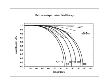
Figure 1: Results of mean field calculations using either the mean field limit ($\gamma_{\bf k}=0$) of the Green’s function program or an exact diagonalization of the corresponding mean field Hamiltonian. Both results are identical. For a monolayer with $S=1$, the magnetization component $\langle S^{z}\rangle$ and the correlation $\langle S^{z}S^{z}\rangle$ in MFT are shown as functions of the temperature for anisotropy coefficients in the range $0<K_{2}<300$; the exchange coupling strength is $J=100$.

In Fig. 1 we show results of mean field (MFT) calculations for $\langle S^{z}\rangle$ and $\langle S^{z}S^{z}\rangle$ as a function of the temperature for different anisotropies in the range of $0<K_{2}<300$ obtained in two ways. The first is an exact diagonalization of the mean field Hamiltonian, which is possible because of its one-body nature. If our Green’s function theory (GFT) for the anisotropy term is exact, calculations with the Green’s function program in the mean field limit (no momentum dependence on the lattice: $\gamma_{\bf k}=0$ of Eq. (12)) should give identical results. This is indeed the case; both results are indistinguishable in Fig. 1. The precise agreement of these very different methods of calculations provides a check on the numerical procedures.

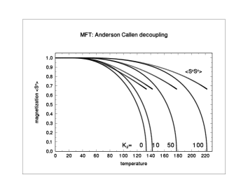
Figure 2: The figure displays results of the MFT limit of a GFT with the Anderson-Callen decoupling, demonstrating the difference from the exact results of Fig. 1. The magnetization $\langle S^{z}\rangle$ and correlation $\langle S^{z}S^{z}\rangle$ are shown only up to $K_{2}=100$, where already the differences are large; results for $K_{2}>100$ lie outside the temperature scale of the figure. Note that the values for $\langle S^{z}S^{z}\rangle=2/3$ contrast with the exact results.

Fig. 2 presents the results of a MFT calculation using the Anderson-Callen decoupling of the single-ion anisotropy terms. The shortcoming of this decoupling is seen by comparing with the exact results of Fig. 1. One observes that, up to $K_{2}=10$, the approximate calculation overshoots the exact one only slightly, but with increasing $K_{2}$ the disagreement becomes worse and worse. The results for $K_{2}>100$ lie outside the frame of the figure.

In the MFT results of Figs. 1 and 2 the well-known shortcoming of MFT is evident, the violation of the Mermin-Wagner theorem: there is a finite Curie temperature for vanishing anisotropy: $T_{Curie}^{MFT}(K_{2}=0)=\frac{4}{3}J=133.33$ for an exchange coupling strength of $J=100$. For arbitrarily large values of the anisotropy, the Curie temperature in MFT is obtained analytically: $T_{Curie}^{MFT}(K_{2}\rightarrow\infty)=S^{2}qJ/(S(S+1))=200$ for $S=1,J=100$ and $q=4$ (q is the coordination number of a square lattice). This limit is almost reached numerically for $K_{2}=300$ as can be seen in Fig. 1.

Our Green’s function theory with the RPA-like treatment of the exchange terms fulfills the Mermin-Wagner theorem: $T_{Curie}\rightarrow 0$ for $K_{2}\rightarrow 0$.

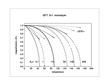
Figure 3: Results of the Green’s function theory (with RPA-like decouplings of the exchange terms) with the same input as in Fig.1 are shown for $\langle S^{z}\rangle$ and $\langle S^{z}S^{z}\rangle$ as functions of the temperature for various anisotropy coefficients $K_{2}$. Note the significant differences from the mean field results of Fig.1.

Comparison of the MFT results of Fig. 1 with the GFT results in Fig. 3 reveals major differences between MFT and GFT with respect to the temperature dependence of $\langle S^{z}\rangle$ for different anisotropies $K_{2}$, particularly in the low temperature region and for small anisotropies. For large anisotropies it can be shown analytically that the full Green’s function theory approaches the MFT limit, $T_{Curie}=200$, when the anisotropy becomes arbitrarily large (see Appendix B). This is physically reasonable because, in the large anisotropy limit, GFT approaches the Ising limit, and, for the Ising model, a RPA treatment is identical with the mean field approach. The results of the exact treatment of the single-ion anisotropy term shown in Fig. 3 represent a significant improvement over the decoupling of this term proposed by Anderson and Callen [13] and the different decoupling of Lines[18], both of which yield a diverging Curie temperature $T_{Curie}\rightarrow\infty$ for $K_{2}\rightarrow\infty$. (See also Appendix B of Ref. [5] in this connection.)

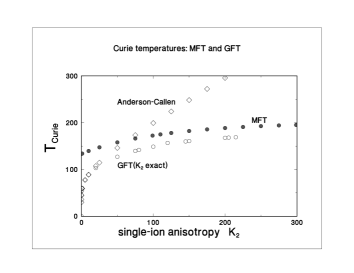
Figure 4: Comparison of the Curie temperatures calculated with the present exact treatment of the anisotropy terms, the Anderson-Callen decoupling[6] and MFT. The first two approaches fulfill the Mermin-Wagner theorem: $T_{C}\rightarrow 0$ for $K_{2}\rightarrow 0$, whereas the MFT result does not. For large anisotropies ($K_{2}\rightarrow\infty$), the new model approaches slowly the mean field results, as it should do, whereas the Anderson-Callen decoupling procedure leads to a diverging $T_{C}$

To show the difference between the new model and the Anderson-Callen decoupling more clearly, we compare in Fig. 4 the Curie temperatures obtained from MFT, the new Green’s function theory, and the Green’s function theory with the Anderson-Callen decoupling of Refs. [5, 6]. For small anisotropies, there is only a slight difference between the two GFT results which, in contrast to MFT, obey the Mermin-Wagner theorem. However, on increasing the anisotropies, the GFT results deviate from one another significantly: for $K_{2}\rightarrow\infty$, the Anderson-Callen result diverges, whereas the exact treatment approaches the MFT limit, albeit very slowly.

The difference between the exact treatment of the anisotropy terms and the approximate Anderson-Callen decoupling is further demonstrated in Fig. 5, where the magnetizations $\langle S^{z}\rangle$ as a function of the temperature for different values of $K_{2}$ are compared. We see that, for small anisotropies, there is rather good agreement, which, however, worsens as $K_{2}$ increases. Another difference concerns the second moments $\langle S^{z}S^{z}\rangle$, which, in the case of the Anderson-Callen decoupling, approach the value $\langle S^{z}S^{z}\rangle(T\rightarrow T_{Curie})=2/3$ (see Ref. [5]), whereas in the exact treatment, the values of $\langle S^{z}S^{z}\rangle(T\rightarrow T_{Curie})$ are larger than $2/3$. This is as it should be, because, as shown in Appendix B, $\langle S^{z}S^{z}\rangle\rightarrow 1$ for $K_{2}\rightarrow\infty$.

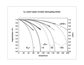
Figure 5: Comparison of GFT calculations for $\langle S^{z}\rangle$ and $\langle S^{z}S^{z}\rangle$ as functions of the temperature using the exact treatment of the anisotropy (open circles) and the Anderson-Callen decoupling used in in Refs. [5, 6] (small dots).

5 Conclusions

We have presented a formal theory for the magnetization of thin ferromagnetic films on the basis of many-body Green’s function theory within a Heisenberg model with anisotropies. The essential improvement over our previous work[5, 6] is the exact treatment of the single-ion anisotropy brought about by the introduction of higher-order Green’s functions. Previously, the anisotropy term was treated by approximate decoupling procedures only at the level of the lowest-order Green’s functions. The exchange interaction terms are decoupled using an RPA-like approach. We did not try to go beyond RPA since our comparison with ‘exact’ quantum Monte Carlo results has shown this to be a very good approximation[15].

Numerical calculations of the magnetization as a function of the temperature for various anisotropies $K_{2}$ (no external field, no dipole-coupling) demonstrate the superiority of the new spin wave model over MFT. In particular, there is no violation of the Mermin-Wagner theorem. The Anderson-Callen decoupling used in our previous work gives results close to those of the new model when the anisotropy $K_{2}$ is small but, as the anisotropy increases, the difference between the two approaches becomes larger: the new model approaches the MFT limit as it should do, whereas the Curie temperature from the Anderson-Callen decoupling diverges.

Our new formulation should allow a future investigation of the reorientation problem when switching on the magnetic field and/or the dipole coupling. The treatment of multi-layer systems and spin $S>1$ should be possible.

We are indebted to A. Ecker and P.J. Jensen for discussions.

Appendix A: The curve-following procedure

Consider a set of $n$ coupled equations characterised by $m$ parameters $\{P_{i};i=1,2\ldots,m\}$ and $n$ variables $\{V_{i};i=1,2,\ldots,n\}$:

$$S_{i}({\bf P}[m];{\bf V}[n])=0,{i=1,\ldots,n}/.$$ (61)

In our case, the parameters are the temperature, the magnetic field components, the dipole coupling strengths, the anisotropy strengths, etc; the variables are the spin-correlations. The coupled equations are obtained by defining the $S_{i}$ from the $n$ self-consistency equations for the correlations vector $\bf v$ (Eq. (48)):

$${\bf S} = {\bf v}-\bf u_{c}^{-1}(R{\cal E}LA+R^{0}L^{0}(u_{c}v-u_{c}^{0})-u_{c}^{0}).$$

For fixed parameters ${\bf P}$, we look for solutions $S_{i}=0$ at localised points, ${\bf V}[n]$, in the n-dimensional space. If now one of the parameters $P_{k}$ is considered to be an additional variable $V_{\circ}$ (in this paper, the temperature is taken as the variable), then the solutions to the coupled equations define curves in the $(n+1)$-dimensional space ${\bf V}[n+1]$. From here on, we denote the points in this space by $\{V_{i};i=0,1,2,...\ldots,n\}$. The curve-following method is a procedure for generating these solution-curves point by point from a few closely-spaced points already on a curve; i.e. the method generates a new solution-point from the approximate direction of the curve in the vicinity of a new approximate point. This is done by an iterative procedure described below. If no points on the curve are known, then an approximate solution point and an approximate direction must be estimated before applying the iterative procedure to obtain the first point on the curve. A second point can then be obtained in the same fashion. If at least two solution-points are available, then the new approximate point can be extrapolated from them and the approximate direction can be taken as the tangent to the curve at the last point.

The iterative procedure for finding a better point, ${\bf V}$, from an approximate point, ${\bf V}^{\circ}$, is now described. One searches for the isolated solution-point in the $n$-dimensional subspace perpendicular to the approximate direction, which we characterise by a unit vector, $\widehat{\bf u}$. The functions $S_{i}$ are expanded up to first order in the corrections about the approximate point, ${\bf V^{\circ}}$:

$$S_{i}({\bf V})=S_{i}({\bf V^{\circ}})+\sum_{j=0}^{n}\frac{\partial S_{i}}{\partial V_{j}}^{\circ}\Delta V_{j},$$ (62)

where $\Delta V_{j}=V_{j}-V_{j}^{\circ}$. At the solution, the $S_{i}$ are all zero, whereas at the approximate point ${\bf V^{\circ}}$ the functions have non-zero values, $S_{i}^{\circ}$; hence, one must solve for the corrections $\Delta V_{j}$ for which the left-hand side in the above equation is zero:

$$\sum_{j=0}^{n}\frac{\partial S_{i}}{\partial V_{j}}^{\circ}\Delta V_{j}=-S_{i}^{\circ};\{i=1,2,\ldots,n\}.$$ (63)

These $n$ equations are supplemented by the constraint requiring the correction to be perpendicular to the unit direction vector:

$$\sum_{j=0}^{n}\widehat{u_{j}}\Delta V_{j}=0.$$ (64)

This improvement algorithm in the subspace is repeated until each of the $S_{i}^{\circ}$ is sufficiently small. In practice we required that $\sum_{i}{(S_{i}^{\circ})^{2}\leq\epsilon}$, where we took $\epsilon=10^{-16}$. If there is no convergence, the extrapolation step-size used to obtain the original ${\bf V}^{\circ}$ is halved, a new extrapolated point obtained, and the improvement algorithm repeated.

The curve-following method is quite general and can be applied to any coupled equations characterised by differentiable functions. By utilizing the information about the solution at neighbouring points, the method is able to find new solutions very efficiently, routinely converging after a few iterations once two starting points have been found.

Appendix B: Curie temperature for $K_{2}\rightarrow\infty$

We show analytically that the Curie temperature of the Green’s function theory with the exact treatment of the anisotropy for a square-lattice monolayer with S=1 approaches the mean field value when the anisotropy coefficient goes to infinity, whereas the Anderson-Callen decoupling leads to a divergence in this limit.

For the case of a single magnetic direction, the $8\times 8$ problem of Eq. (10) reduces to a $2\times 2$ problem for the Green’s functions $G_{ij}^{+,-}=\langle\langle S_{i}^{+};S_{j}^{-}\rangle\rangle$ and $G_{ij}^{z+,-}=\langle\langle(2S_{i}^{z}-1)S_{j}^{+};S_{j}^{-}\rangle\rangle$. For this special case, it is possible to derive analytical expressions for the correlations $\langle S^{z}\rangle$ and $\langle S^{z}S^{z}\rangle$:

$$\langle S^{-}S^{+}\rangle = 2-\langle S^{z}\rangle-\langle S^{z}S^{z}\rangle=\frac{1}{\pi^{2}}\int_{0}^{\pi}dk_{x}\int_{0}^{\pi}dk_{y}\Big{\{}\frac{1}{\omega^{+}-\omega^{-}}$$ (65)

$$\Big{[}(2\langle S^{z}\rangle(\omega^{+}-\langle S^{z}\rangle J_{0})+K_{2}(6\langle S^{z}S^{z}\rangle-4))\frac{1}{e^{\beta\omega^{+}}-1}$$

$$-(2\langle S^{z}\rangle(\omega^{-}-\langle S^{z}\rangle J_{0})+K_{2}(6\langle S^{z}S^{z}\rangle-4))\frac{1}{e^{\beta\omega^{-}}-1}\Big{]}\Big{\}}$$

$$\langle S^{-}(2S^{z} - 1)S^{+}\rangle=\langle S^{z}\rangle-\frac{1}{2}(6\langle S^{z}S^{z}\rangle-4)=\frac{1}{\pi^{2}}\int_{0}^{\pi}dk_{x}\int_{0}^{\pi}dk_{y}\Big{\{}\frac{1}{\omega^{+}-\omega^{-}}$$ (66)

$$\Big{[}((6\langle S^{z}S^{z}\rangle-4)(\omega^{+}-\langle S^{z}\rangle J_{0})+K_{2}(2\langle S^{z}\rangle))\frac{1}{e^{\beta\omega^{+}}-1}$$

$$-((6\langle S^{z}S^{z}\rangle-4)(\omega^{-}-\langle S^{z}\rangle J_{0})+K_{2}(2\langle S^{z}\rangle))\frac{1}{e^{\beta\omega^{-}}-1}\Big{]}\Big{\}}$$

with

$$\omega^{\pm}=\frac{1}{2}\langle S^{z}\rangle(J_{0}-J_{\bf k})\pm\sqrt{K_{2}^{2}-\frac{1}{2}(6\langle S^{z}S^{z}\rangle-4)K_{2}J_{\bf k}-\frac{1}{4}\langle S^{z}\rangle^{2}}.$$ (67)

At the Curie temperature, $\langle S^{z}\rangle\rightarrow 0$, so that the equation for $\omega^{\pm}$ becomes

$$\omega^{\pm}(\langle S^{z}\rangle=0)=\pm\omega^{0}=\pm\sqrt{K_{2}(K_{2}-\frac{1}{2}(6\langle S^{z}S^{z}\rangle)-4)J_{\bf k})},$$ (68)

Equation (65) then reduces to

$$2-\langle S^{z}S^{z}\rangle=(6\langle S^{z}S^{z}\rangle-4)\frac{1}{\pi^{2}}\int_{0}^{\pi}dk_{x}\int_{0}^{\pi}dk_{y}\frac{K_{2}}{2\omega^{0}}\coth(\beta\omega^{0}/2).$$ (69)

For large $K_{2}$, $\omega^{0}=K_{2}\sqrt{1-(6\langle S^{z}S^{z}\rangle-4)J_{\bf k}/(2K_{2})}\simeq K_{2}$. Passing to the limit $K_{2}\rightarrow\infty$, one obtains from Eq. (69) at $T_{Curie}$

$$\langle S^{z}S^{z}\rangle=1.$$ (70)

Now, expanding Eq. (66) around $\langle S^{z}\rangle=0$, and comparing the coefficients of $\langle S^{z}\rangle$ of the resulting equation, one has at $T_{Curie}$

$$1=\frac{1}{\pi^{2}}\int_{0}^{\pi}dk_{x}\int_{0}^{\pi}dk_{y} \Big{\{}(\frac{K_{2}}{\omega^{0}}-\frac{J_{\bf k}(6\langle S^{z}S^{z}\rangle-4)}{4\omega^{0}})\coth(\frac{\beta\omega^{0}}{2})$$ (71)

$$+ (\frac{1}{2}J_{\bf k}-J_{0})\beta(6\langle S^{z}S^{z}\rangle-4)\frac{e^{\beta\omega^{0}}}{(e^{\beta\omega^{0}}-1)^{2}}\Big{\}}.$$

Noting that $\int_{0}^{\pi}dk_{x}\int_{0}^{\pi}dk_{y}J_{\bf k}=0$ and that $\omega^{0}\simeq K_{2}$ for large $K_{2}$, one obtains from Eq. (71)

$$1-\coth(\frac{\beta K_{2}}{2})=-J_{0}\beta(6\langle S^{z}S^{z}\rangle-4))\frac{e^{\beta K_{2}}}{(e^{\beta K_{2}}-1)^{2}}.$$ (72)

Again, goint to the limit $K_{2}\rightarrow\infty$ and using Eq. (70), one obtains for the Curie temperature

$$T_{Curie}=J_{0}\frac{1}{2}(6\langle S^{z}S^{z}\rangle-4)=J_{0}=4J$$ (73)

This is just the MFT result! This is physically reasonable because a large anisotropy approaches the Ising limit, and the RPA for the Ising model is identical to its mean field treatment.

This is in contrast to the result of the decoupling procedure. In Appendix B of Ref. [5] we have shown that the Anderson-Callen decoupling of the anisotropy term leads for a square monolayer to a Curie temperature

$$T_{Curie}\simeq\frac{8\pi J/3}{\ln(1+3\pi^{2}J/K_{2})},$$ (74)

which diverges for $K_{2}\rightarrow\infty$!

References

[1] R.Sellmann, H. Fritzsche, H. Maletta, V. Leiner, and R.
Siebrecht, Phys. Rev. B 64 (2001) 054418
[2] S. Pütter, H.F. Ding, Y.T. Millev, H.P. Oepen, and J.
Kirschner, Phys. Rev. B 64 (2001) 092409
[3] A. Moschel, K.D. Usadel, Phys. Rev. B 49 (1994)
12868;
P.J. Jensen, K.H. Bennemann, in ’Magnetism and Electronic Correlations in
Local-Moment Systems: Rare-Earth Elements and Compounds’, ed. M. Donath, P.A.
Dowben, and W. Nolting, (World Scientific, 1998), p. 113-141
[4] P.J. Jensen, K.H. Bennemann, Solid State Comm. 100
(1996) 585, ibid. 105 (1998) 577; A. Hucht, K.D. Usadel, Phys. Rev. B
55 (1997) 12309
[5] P. Fröbrich, P.J. Jensen, P.J. Kuntz, Eur. Phys. J. B
13 (2000) 477
[6] P. Fröbrich, P.J. Jensen, P.J. Kuntz, A. Ecker, Eur. Phys.
J. B 18 (2000) 579