Granular and Nano-Elasticity

Abstract

The modeling of the elastic properties of granular or nanoscale systems requires the foundations of the theory of elasticity to be revisited, as one explores scales at which this theory may no longer hold. The only cases for which a microscopic justification of elasticity exists are (nearly) uniformly strained lattices. A microscopic theory of elasticity, as well as simulations, reveal that standard continuum elasticity applies only at sufficiently large scales (typically 100 particle diameters). Interestingly, force chains, which have been observed in experiments on granular systems, and attributed to non-elastic effects, are shown to exist in systems composed of harmonically interacting constituents. The corresponding stress field, which is a continuum mechanical (averaged) entity, exhibits no chain structures even at near-microscopic resolutions, but it does reflect macroscopic anisotropy, when present.

,

1 Introduction

It is quite surprising that the existing microscopic justification of the time-honored theory of elasticity, which has been thoroughly researched in a variety of disciplines, is limited to lattice atomic configurations [1]. Classical continuum elasticity theory has been applied to a large variety of systems, including granular materials [2]. In recent years the same theory has been applied for the description of elastic properties of micro- and nano-scale systems (e.g., [3]). It is a-priori unclear whether this theory applies at such small scales.

The study presented below shows that the justification of elastic theory based on a ‘microscopic’ picture is not entirely straightforward. In fact, we show that continuum elasticity is limited to sufficiently large scales. One of the other results presented in this paper is that ‘force chains’ in granular systems, which have been attributed by some authors to non-elastic effects [4], are reproduced in simulations of elastic systems, in good agreement with experiments.

2 Coarse Graining and Constitutive Relations

2.1 Preliminaries

Below the term ‘particles’ is taken to mean grains in a granular system or atoms in a solid. Classical mechanics is assumed throughout this paper. Following [5] define, for a system of particles, the coarse grained mass and momentum densities, at the position ${\bf r}$ and time $t$, by $\rho({\bf r},t)\equiv\sum_{i}m_{i}\phi[{\bf r}-{\bf r}_{i}(t)]$ and ${\bf p}({\bf r},t)\equiv\sum_{i}m_{i}{\bf v}_{i}(t)\phi[{\bf r}-{\bf r}_{i}(t)]$, respectively, where $\{{\bf r}_{i}(t);{\bf v}_{i}(t);m_{i}\}$ are the positions, velocities and masses of the particles, indexed by $i$, and $\phi({\bf R})$ is a normalized non-negative coarse graining function (with a single maximum at ${\bf R}=0$) of width $\lambda$, the coarse graining scale. The velocity field is defined by ${\bf V}({\bf r},t)\equiv{\bf p}({\bf r},t)/\rho({\bf r},t)$. Upon taking the time derivatives of these coarse grained fields and performing straightforward algebraic manipulations [5] one obtains the equation of continuity, as well as the momentum conservation equation: $\dot{p}_{\alpha}({\bf r},t)=-\frac{\partial}{\partial r_{\beta}}\left[\rho({\bf r},t)V_{\alpha}({\bf r},t)V_{\beta}({\bf r},t)-\sigma_{\alpha\beta}({\bf r},t)\right]$, where Greek indices denote Cartesian coordinates. The stress tensor, $\sigma_{\alpha\beta}$, is composed of a kinetic contribution, irrelevant for our purposes (we consider quasi-static deformations), and a “contact” contribution. Neglecting the former, one obtains:

$$\sigma_{\alpha\beta}({\bf r},t)=-\frac{1}{2}\sum_{i,j;i\neq j}f_{ij\alpha}(t){r}_{ij\beta}(t)\int_{0}^{1}ds\phi[{\bf r}-{\bf r}_{i}(t)+s{\bf r}_{ij}(t)].$$ (1)

where $f_{ij\alpha}(t)$ is the $\alpha$-th component of the force exerted on particle $i$ by particle $j$ ($j\neq i$) at time $t$ (assuming pairwise interactions) and $r_{ij\alpha}\equiv r_{i\alpha}-r_{j\alpha}$.

2.2 Displacement and Strain

Following elementary continuum mechanics, the velocity of a material particle whose initial (Lagrangian) coordinate is ${\bf R}$ satisfies: ${\bf V}^{\rm La}({\bf R},t)=\partial{{\bf u}^{\rm La}\left({\bf R},t\right)}/\partial{t}$, where ${\bf u}^{\rm La}({\bf R},t)\equiv{\bf r}({\bf R},t)-{\bf R}$ is the (Lagrangian) displacement field. Therefore: ${\bf u}^{\rm La}({\bf R},t)=\int_{0}^{t}{\bf V}^{\rm La}({\bf R},t^{\prime})dt^{\prime}$. Using the definitions presented in Sec. 2.1, it follows that:

$${\bf u}^{\rm La}({\bf R},t)\equiv\int_{0}^{t}\frac{\sum_{i}m_{i}{\bf v}_{i}(t^{\prime})\phi[{\bf r}({\bf R},t^{\prime})-{\bf r}_{i}(t^{\prime})]}{\sum_{j}m_{j}\phi[{\bf r}({\bf R},t^{\prime})-{\bf r}_{j}(t^{\prime})]}dt^{\prime}.$$ (2)

Noting that $\dot{{\bf u}}_{i}={\bf v}_{i}$, where ${\bf u}_{i}$ is the displacement of particle $i$, and invoking integration by parts in Eq. (2), one obtains:

$${\bf u}({\bf r},t)\simeq\frac{\sum_{i}m_{i}{\bf u}_{i}(t)\phi[{\bf r}-{\bf r}_{i}(t)]}{\sum_{j}m_{j}\phi[{\bf r}-{\bf r}_{j}(t)]}+\mbox{``non-linear terms''},$$ (3)

where the result has been translated to the Eulerian representation. The correction terms can be shown to beget non-linear terms in the constitutive relations. The linear strain is given by $\epsilon_{\alpha\beta}({\bf r},t)\equiv\frac{1}{2}\left[\frac{\partial u_{\alpha}({\bf r},t)}{\partial r_{\beta}}+\frac{\partial u_{\beta}({\bf r},t)}{\partial r_{\alpha}}\right]$. Note that the exact displacement and strain obtained here are different from the commonly defined mean field strain, cf. e.g. [6]. Mean field theories are based on the assumption that the relative particle displacements are described by the macroscopic strain, $u_{ij\alpha}({\bf r},t)=\epsilon_{\alpha\beta}R_{ij\beta}$, where ${\bf u}_{ij}\equiv{\bf u}_{i}-{\bf u}_{j}$. A suggested improvement is the “best fit” strain [7]. These mean field approaches are inaccurate and often lead to incorrect constitutive relations [8].

2.3 Stress-Strain Relation

The microscopic expressions for the stress [Eq. (1)] and the strain are not manifestly proportional. Therefore elasticity is not a-priori obvious. To see how it still comes about, consider the case of harmonic (and local) pairwise particle potentials $U_{ij}=\frac{1}{2}K_{ij}\left(|r_{ij}|-l_{ij}\right)^{2}$. The forces are then given, to linear order in $\delta{\bf r}_{ij}\equiv{\bf u}_{ij}$, by ${\bf f}_{ij}=-K_{ij}\left(\hat{{\bf r}}^{0}_{ij}\cdot\delta{\bf r}_{ij}\right)\hat{{\bf r}}^{0}_{ij}$. The stress [Eq. (1)] is then given by $\sigma_{\alpha\beta}^{\mathrm{lin}}({\bf r},t)=\frac{1}{2}\sum_{ij}K_{ij}\hat{r}^{0}_{ij\gamma}\delta r_{ij\gamma}\hat{r}^{0}_{ij\alpha}{r}^{0}_{ij\beta}\phi({\bf r}-{\bf r}^{0}_{i})$, up to nonlinear terms in $\left\{\delta{\bf r}_{ij}\right\}$. The superscript $0$ denotes the reference configuration.

Consider a volume $\Omega$ which is much larger than the coarse graining scale, $\lambda$, and let ${\bf r}$ be an interior point of $\Omega$ which is ‘far’ from its boundary. Let upper case Latin indices denote the particles in the exterior of $\Omega$ which interact with particles inside $\Omega$. Since the considered system is linear, there exists a Green’s function $\bf G$ such that $u_{i\alpha}=G_{i\alpha J\beta}u_{J\beta}$ for $i\in\Omega$. Hence, $u_{ij\alpha}=\left(G_{i\alpha J\beta}-G_{j\alpha J\beta}\right)u_{J\beta}$. When all ${\bf u}_{J}$ are equal (rigid translation), ${\bf u}_{ij}=0$. Hence, $u_{ij\alpha}=\left(G_{i\alpha J\beta}-G_{j\alpha J\beta}\right)\left[u_{J\beta}-u_{\beta}({\bf r})\right]$. Define $L_{ij\alpha J\beta}\equiv G_{i\alpha J\beta}-G_{j\alpha J\beta}$. One then obtains $u_{ij\alpha}=L_{ij\alpha J\beta}\left[u_{\beta}({\bf r}_{J})-u_{\beta}({\bf r})\right]+L_{ij\alpha J\beta}\left[u_{J\beta}-u_{\beta}({\bf r}_{J})\right]$, where $u_{J\beta}-u_{\beta}({\bf r}_{J})$ is a fluctuating displacement. The sum over $J$ in the second term can be shown to be subdominant when the linear size of the volume $\Omega$ greatly exceeds the coarse graining scale. Furthermore, to lowest order in a gradient expansion, $u_{\beta}({\bf r}_{J})-u_{\beta}({\bf r})\simeq\frac{\partial u_{\beta}({\bf r})}{\partial r_{\gamma}}\left(r_{J\gamma}-r_{\gamma}\right)$. Substituting this result in $\mbox{\boldmath{$\sigma$}}^{\mathrm{lin}}$, and employing rotational symmetry, one obtains:

$$\sigma_{\alpha\beta}({\bf r})\simeq\frac{1}{2}\epsilon_{\mu\nu}({\bf r})\sum_{ij}K_{ij}L_{ij\gamma J\mu}\left(r^{0}_{J\nu}-r_{\nu}\right)\hat{r}^{0}_{ij\alpha}{r}^{0}_{ij\beta}\hat{r}^{0}_{ij\gamma}\phi({\bf r}-{\bf r}^{0}_{i}).$$ (4)

Thus linear elasticity is valid when $\left|\lambda\nabla_{\alpha}\nabla_{\beta}{\bf u}\right|\ll 1$ and $\left\|\mbox{\boldmath{$\epsilon$}}\right\|\ll 1$. Note that the elastic moduli depend, in principle, on the position as well as the resolution (through the coarse graining function $\phi$).

3 Numerical Results

In order to study the crossover from microelasticity to macroelasticity [9], we have considered a two dimensional (2D) rectangular slab, composed of uniform disks (of diameter $d$) whose centers are positioned on a triangular lattice, with nearest neighbors coupled by uniform linear springs (of rest length $d$), and a three dimensional (3D) slab, composed of uniform spheres (of diameter $d$) with springs coupling nearest-neighbors (spring constant $K_{1}$) and next-nearest-neighbors ($K_{2}$). Both systems can be shown to correspond to isotropic elastic media in the continuum limit [1] (for the 3D system, only if $K_{1}=K_{2}$). The particles at the bottom layer are attached to a rigid floor, and a downward force is applied to the central particle in the top layer. This is intended for comparison with 2D [10] and 3D [11] granular experiments (even though these models do not directly describe the interaction of granular particles and are primarily intended for studying the crossover between microelasticity and macroelasticity, they closely reproduce some of the experimental results). Fig. 1 presents a comparison between the vertical stress exerted on the floor of the system for different slab heights (numbers of layers of particles) and continuum elastic solutions, for both systems ($K_{1}=K_{2}$ for the 3D system). The convergence to the appropriate (rough rigid support) elastic stress distribution for a sufficient number of layers is evident.

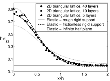
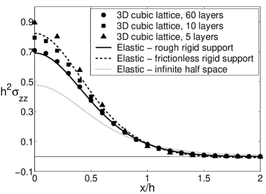
Figure 1: The vertical stress at the bottom of a 2D triangular lattice (left) and a 3D cubic lattice (right), compared to continuum elastic solutions. The results are scaled by the slab height $h$.

The observation of “force chains” in experiments [10] and simulations [12] has been interpreted as evidence for non-elastic effects [4]. However, in a plot of the interparticle forces in the 2D system described above (Fig. 2, left) one can identify “force chains” though the microscopic interactions are strictly linear, and the large scale behavior corresponds to isotropic elasticity. The corresponding distribution of interparticle forces [9] closely resembles the experimental findings of Geng et al. [10]. The $zz$ component of the stress field, calculated using Eq. (1) with a Gaussian coarse graining function [5] of width $d$ (i.e., with fine resolution), is shown in Fig. 2, on the right. The force chains are not evident any more. The force chains result from the microscopic anisotropy dictated by the fact that a single particle is never subject to an isotropic force distribution. However, even at small, but finite, spatial resolution, the calculation of the stress tensor inherently involves averaging over the forces acting on the particles, so that this anisotropy does not appear in the stress field. Similar results [9] are obtained for random 2D systems.

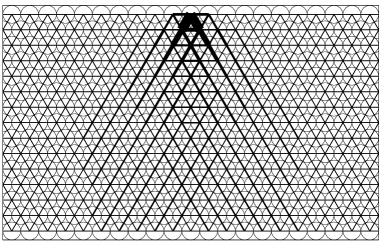
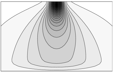
Figure 2: Left: Force chains in a 2D triangular lattice. A vertical force is applied to the center particle in the top layer. The line widths are proportional to the forces. Only the central region of the lattice is shown (the lattice comprises $15\times 41$ particles). Right: Contour plot of the vertical stress component, $\sigma_{zz}$, in the same region.

A more realistic model with unilateral (“one-sided”) springs, active only upon compression, yields results which are even closer to the experiments [9]. In this case, some of the springs are disconnected (as obtained in [13] for a pile geometry) when the external force is applied. In particular, the horizontal springs in a triangular region below the point of application of the force are severed, and the corresponding macroscopic properties are anisotropic. The resulting stress distribution [9] is similar to that predicted by hyperbolic models of force propagation [4], but it is a result of an elastic model.

References

- [1] C. Kittel, Introduction to Solid State Physics (Second Edition) (Wiley, 1956); R. P. Feynman, R. B. Leighton, and M. Sands, The Feynman Lectures on Physics, Vol. II (Addison-Wesley, 1964); M. Born and K. Huang, Dynamical Theory of Crystal Lattices (Clarendon Press, 1954).
- [2] S. B. Savage, in Proc. NATO ASI on Physics of Dry Granular Media, Cargèse, France, 1997, edited by H. J. Herrmann, J. P. Hovi, and S. Luding, pp. 25–95, Kluwer, 1998; R. M. Nedderman, Statics and Kinematics of Granular Materials (Cambridge University Press, 1992).
- [3] J. Schiøtz et al., Phys. Rev. B 60, 11971 (1999); A. G. Khachaturyan, S. Semenovskaya, and T. Tsakalakos, Phys. Rev. B 52, 15909 (1995); R. Lifshitz and M. L. Roukes, Phys. Rev. B 60, 5600 (2000).
- [4] M. E. Cates, J. P. Wittmer, J.-P. Bouchaud, and P. Claudin, Chaos 9, 511 (1999); J.-P. Bouchaud, P. Claudin, D. Levine, and M. Otto, Eur. Phys. J. E 4, 451 (2001).
- [5] B. J. Glasser and I. Goldhirsch, Physics of Fluids 13, 407 (2001).
- [6] R. J. Bathurst and L. Rothenburg, Journal of Applied Mechanics 55, 17 (1988).
- [7] C.-L. Liao, T.-P. Chang, D.-H. Young, and C. S. Chang, Int. J. Solids and Structures 34, 4087 (1997).
- [8] C. Goldenberg and I. Goldhirsch, Unpublished.
- [9] C. Goldenberg and I. Goldhirsch, cond-mat/0108297.
- [10] A. Drescher and G. de Josselin de Jong, J. Mech. Phys. Solids 20, 337 (1972); J. Geng et al., Phys. Rev. Lett. 87, 035506 (2000).
- [11] G. Reydellet and E. Clément, Phys. Rev. Lett. 86, 3308 (2001); D. Serero et al., Eur. Phys. J. E 6, 169 (2001).
- [12] P. A. Cundall and O. D. L. Strack, Geotechnique 29, 47 (1979); F. Radjai, S. Roux, and J. J. Moreau, Chaos 9, 544 (1999).
- [13] S. Luding, Phys. Rev. E 55, 4720 (1997).