BKT transition and level spectroscopy

Abstract

Berezinskii-Kosterlitz-Thouless (BKT) transition is one of the instability mechanisms for the Tomonaga-Luttinger liquid. But in the BKT transition, there are logarithmic-correction problems, which make it very difficult to treat BKT transitions numerically. We propose a method, “level spectroscopy”, to overcome such difficulties, based on the renormalization group analysis and the symmetry consideration.

1 Introduction

Tomonaga-Luttinger (TL) liquid [1, 2] is an important concept for one dimensional (1D) quantum systems (spin, electron systems, nanotube, etc. at $T=0$) with the continuous symmetry (U(1),SU(2), etc.), and TL liquid is closely related to several 2D classical models (6-vertex model, classical XY spin, superconducting film, roughening transition, etc. at $T\neq 0$). Therefore, it becomes crucial to understand instabilities of TL liquid.

One of the instabilities of TL liquid is the Berezinskii-Kosterlitz-Thouless (BKT) transition [3, 4, 5]. Although the BKT transition has been well known, it has not been recognized that there are pathological problems to analyze numerically BKT transitions. One of these problems is that the finite size scaling technique [6], which is successful for second order transitions, can not be applied for BKT transitions [7, 8], since there are logarithmic corrections from the marginal coupling. Recently, combining the renormalization group calculation and the symmetry, we have developed a remedy, “level spectroscopy”, to overcome these difficulties.

In the next section, we compare the BKT transition with the second order transition. In §3, we introduce the concept of the level spectroscopy and how to use it. In §4, we deduce the level spectroscopy from the sine-Gordon model, which is an effective model to describe the BKT transition. For readers who are not familiar with the sine-Gordon model, we recommend to read §5 (physical examples) before §4.

2 BKT transition versus second order transition

First, we briefly review the renormalization concept. Let us consider a $d$-dimensional classical Hamiltonian (or an action for a $(d-1)+1$ dimensional quantum system) [9]

$$H=H_{0}+\sum_{j}y_{j}\int\psi_{j}(x)\frac{d^{d}x}{\alpha^{d}},$$ (1)

where $H_{0}$ is scale invariant, $\psi_{j}(x)$ is a local order parameter, $y_{j}$ is an effective coupling constant (or some external field), $\alpha$ is a short-range cutoff.

When changing a scale as $\alpha^{\prime}=b\alpha$, effective local order parameters change as $\psi^{\prime}_{j}=b^{x_{j}}\psi_{j}$ ($x_{j}$: scaling dimension) and according to this, effective couplings change as $y^{\prime}_{j}=b^{d-x_{j}}y_{j}$. If $y_{j}=0$, then $y^{\prime}_{j}$ remain 0 (fixed point). We call the case $y^{\prime}_{j}$ diverging for $b\rightarrow\infty$ (i.e. $x_{j}<d$) as relevant, whereas the case $y^{\prime}_{j}$ converging (i.e. $x_{j}>d$) as irrelevant.

At the fixed point, the system is scale invariant, therefore the correlation length is infinite $\xi=\infty$. Although regions which flow into the fixed point are not strictly scale invariant, $\xi=\infty$ in these regions (critical regions).

For the infinitesimal scale transformation $\alpha^{\prime}=\alpha e^{dl}\approx\alpha(1+dl)$, one can treat eq. (1) perturbatively.

2.1 Second order transition

The scaling equations for second order transitions are

$$\frac{dy_{j}(l)}{dl}=(d-x_{j})y_{j}(l)\equiv\beta_{j}(\{y_{j}(l)\})\qquad(l\equiv\ln(L),L:{\rm system\;size}).$$ (2)

As an example, let us consider the two scaling field case. When $\psi_{1}$ is a relevant operator and $\psi_{2}$ is an irrelevant one, the renormalization group flow is given in Fig. 1 a.

Since the second order transition occurs where the sign of the $\beta$ function (for a relevant coupling $y_{1}$) changes, one can use this fact to determine the critical point [6].

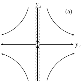
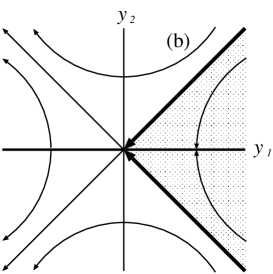
Figure 1: Renormalization flows for (a) second order transition, (b) BKT transition. Shaded parts are critical region.

2.2 BKT transition

The BKT transition ($d=2$) is described by the following RG equation [5]

$$\framebox{$\displaystyle\frac{dy_{1}(l)}{dl}=-y_{2}(l)^{2},\;\frac{dy_{2}(l)}{dl}=-y_{1}(l)y_{2}(l)$},$$ (3)

where fixed points are $y_{2}=0$. All of the points in $|y_{2}|<y_{1}$ are renormalized to $y_{2}=0$, thus in this region correlation lengths are infinite ($\xi=\infty$) or massless. Other regions are massive ($\xi$ finite), except $y_{2}=0$ (see Fig 1 b). We call the region within $|y_{2}|<y_{1}$ as the massless region, the lines $y_{2}=\pm y_{1}$ as the BKT critical lines, $y_{1}=0$ as the Gaussian fixed line. The point $y_{1}=y_{2}=0$ has a special meaning (two BKT lines and one Gaussian line intersect), and we call it as the BKT multicritical point.

Note that on the BKT line, the coupling $y_{1}$ is marginal (i.e. $x_{1}=2$) and it behaves as $y_{1}(l)=1/l=1/\ln(L)$. Another important fact is that on the Gaussian fixed line ($y_{2}=0$), the scaling dimension of $\psi_{2}$ is varying with $y_{1}$.

2.3 Comparison between second order and BKT transition

1. Critical region ($\xi=\infty$) is isolated in the second order transition, whereas it is extended in the BKT transition.

2. Zero point of the $\beta$ function corresponds to the critical point in the second order transition, whereas for the BKT, it has no special meaning.

3. Since the renormalization group behavior on BKT critical lines ($y_{2}=\pm y_{1}$) is marginal, there appear logarithmic corrections $1/\ln(L)$, e.g., in the correlation function as [5]

   $$r^{1/4}(\ln r)^{1/8},$$ (4)

   or in the energy gap for the finite size system as [10, 11]

   $$\Delta E(L)=\frac{2\pi v}{L}\frac{1}{8}\left(1-\frac{1}{2}\frac{1}{\ln L}\right),$$

   therefore finite size effects are very large.

All of them make it very difficult to treat the BKT transition numerically (N.B. universal jump is also affected by logarithmic corrections, but O($1/(\ln L)^{2}$)).

3 Level spectroscopy

The BKT transition occurs where some physical quantities change from irrelevant to relevant. Thus it is useful to investigate scaling dimensions near marginal. In fact, on the Gaussian line (i.e., without interaction), several scaling dimensions cross at the BKT multicritical point (see Fig. 2 a, or eqs. (17), (18)).

Based on the conformal field theory (CFT) in 2D [12], one can obtain the scaling dimensions using the energy gap for the finite system. The relation between the energy gap $\Delta E_{j}$ of the system size $L$ and the scaling dimension $x_{j}$ is [9, 13]

$$\framebox{$\displaystyle\Delta E_{j}=\frac{2\pi vx_{j}}{L}$},$$ (5)

where $v$ corresponds with a renormalized Fermi velocity, or a spin wave velocity.

Each excitation can be classified by quantum numbers ($m$ (magnetization or electron density, related with U(1) symmetry), $P$ (parity), $q$ (wave number)).

In the normal BKT transition, there is no symmetry breaking in the massive phase. But in general, the BKT transition may be combined with a discrete symmetry, and there occurs a $Z_{p}$ discrete symmetry breaking in the massive phase.

Procedure to use level spectroscopy

1. Classification of BKT transitions with the discrete symmetry

   1. BKT transition without symmetry breaking (§3.1, §3.3)

      (e.g. 2D classical XY, integer $S$ XXZ quantum spin chain )

      From table 1, choose the excitation with some quantum numbers, then from the level crossing, determine BKT transition line.

   2. BKT transition with the $Z_{2}$ symmetry breaking (§3.2)

      (e.g. 6 vertex model, half-integer $S$ XXZ quantum spin chain )

      From table 2, choose the excitation with some quantum numbers, then from the level crossing, determine BKT transition line.

   3. BKT transition with the $Z_{p}$ ($p>2$ integer) symmetry breaking

      (e.g. 2D $p$-state clock model)

      Although we do not explain the $Z_{p}$ case here, this case has been discussed in [14]. Note that there is a difference for $p$ even or odd case.

2. Checking of the universality class (elimination of logarithmic corrections)

   1. Scaling dimension (§3.4)

      From tables 1, 2, choose the excitations eliminating logarithmic corrections each other, and check the universality class.

   2. Central charge $c=1$ (§3.5)

3.1 Normal BKT transition

In the normal BKT transition, there is no symmetry breaking. In table 1, we show the relation between the scaling dimension (or excitation (5)) and quantum numbers [14]. In the neighborhood of the scaling dimension $x=2$, on the BKT line $y_{2}(l)=\pm y_{1}(l)$, there is a level crossing of excitations with quantum numbers ($m=\pm 4,P=1,q=0$) and ($m=0,P=1,q=0$) (see table 1, Fig. 2), thus we can determine the BKT transition line.

Next, since the ratios of logarithmic corrections ($1/\ln L$) on the BKT transition line are $2:1:-1$ (corresponding to $x_{0,cos},x_{0,sin},x_{\pm 4,0}$ in table 1), we can eliminate logarithmic corrections and check the universality class.

This level crossing on the BKT transition reflects the (hidden) SU(2) symmetry [20], thus it is correct up to higher order loops. We can see this SU(2) symmetry explicitly, including the twisted boundary condition (see §3.3).

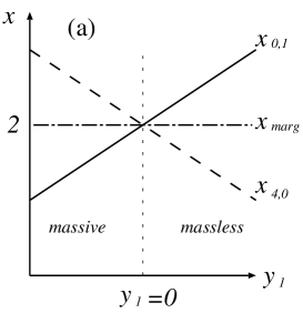
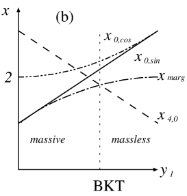
Figure 2: Scaling dimension $x$ in the neighborhood of BKT transition (a) $y_{2}=0$ (on the Gaussian fixed line) (b) $y_{2}\neq 0$.

m	P	q	BC	$x$	operator in s.G.	abbr.
$\pm 2$	1	0	PBC	$1/2-y_{1}(l)/4$	$\exp(\pm i2\sqrt{2}\theta)$	$x_{\pm 2,0}$
0	$-1^{*}$		TBC	$1/2+y_{1}(l)/4-y_{2}(l)/2$	$\sin(\phi/\sqrt{2})$	$x_{0,sin}^{TBC}$
0	$1^{*}$		TBC	$1/2+y_{1}(l)/4+y_{2}(l)/2$	$\cos(\phi/\sqrt{2})$	$x_{0,cos}^{TBC}$
$\pm 4$	1	0	PBC	$2-y_{1}(l)$	$\exp(\pm i4\sqrt{2}\theta)$	$x_{\pm 4,0}$
0	1	0	PBC	$2-y_{1}(l)(1+4t/3)$	marginal	$x_{marg}$
0	-1	0	PBC	$2+y_{1}(l)$	$\sin(\sqrt{2}\phi)$	$x_{0,sin}$
0	1	0	PBC	$2+2y_{1}(l)(1+2t/3)$	$\cos(\sqrt{2}\phi)$	$x_{0,cos}$

Table 1: Renormalized scaling dimensions $x$ and quantum numbers ($m,P,q$) for the normal BKT transition. PBC denotes periodic boundary condition, TBC twisted boundary condition. $t$ is a distance from the BKT critical line, defined as $y_{2}(l)=\pm y_{1}(l)(1+t)$. Couplings $y_{1},y_{2}$ follow renormalization group equations (3), and on the BKT transition line $y_{1}(l)=\pm y_{2}(l)=1/\ln(L/L_{0})$.

3.2 BKT transition with $Z_{2}$ symmetry breaking

Next we consider the BKT transition coupled with a discrete symmetry. Especially in the BKT transition with the $Z_{2}$ symmetry breaking (in the massive region), the level crossing of the lowest excitations in each region corresponds to the phase boundary.

We introduce a quantum number corresponding to the $Z_{2}$ symmetry (wave number $q=0,\pi$ etc.). In table 2 we summarize quantum numbers and excitations [15, 16]. Level crossings on BKT transition lines can be observed not only $x=2$ (N. B. quantum numbers differ from table 1), but also $x=1/2$, where the excitations with quantum numbers ($m=0,q=\pi,P=\pm 1$) and ($m=\pm 1$) show a level crossing (Fig. 3 a, table 2).

About the Gaussian fixed line $y_{2}=0$, each of the $Z_{2}$ symmetry broken massive phases has different parity, thus it occurs a level crossing of excitations $m=0,q=\pi,P=\pm 1$ (Fig. 3 b).

m	P	q	$x$	operator in s.G.	abbr.
$\pm 1$			$1/2-y_{1}(l)/4$	$\exp(\pm i\sqrt{2}\theta)$	$x_{\pm 1,0}$
0	-1	$\pi$	$1/2+y_{1}(l)/4-y_{2}(l)/2$	$\sin(\sqrt{2}\phi)$	$x_{0,sin}$
0	1	$\pi$	$1/2+y_{1}(l)/4+y_{2}(l)/2$	$\cos(\sqrt{2}\phi)$	$x_{0,cos}$
$\pm 2$	1	0	$2-y_{1}(l)$	$\exp(\pm i2\sqrt{2}\theta)$	$x_{\pm 2,0}$
0	1	0	$2-y_{1}(l)(1+4t/3)$	marginal	$x_{marg}$
0	-1	0	$2+y_{1}(l)$	$\sin(2\sqrt{2}\phi)$	$x_{0,sin2}$
0	1	0	$2+2y_{1}(l)(1+2t/3)$	$\cos(2\sqrt{2}\phi)$	$x_{0,cos2}$

Table 2: Renormalized scaling dimensions $x$ and quantum numbers ($m,P,q$) for BKT transition with $Z_{2}$ symmetry.

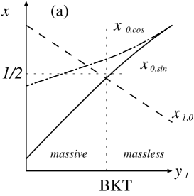
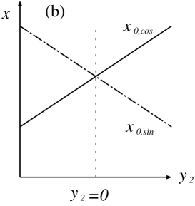
Figure 3: Scaling dimensions $x$ for BKT transition with $Z_{2}$ symmetry. (a) Near the BKT transition line ($y_{2}>0$ case) (b) Near the Gaussian fixed line.

3.3 Twisted boundary condition (TBC)

In the previous section case, one can distinguish two massive phases on the both side of the Gaussian fixed line, by using $Z_{2}$ symmetry. How to distinguish two massive phases in the normal BKT transition? Using the twisted boundary condition (TBC) method [17, 18], we can clarify the hidden $Z_{2}\times Z_{2}$ symmetry.

TBC is expressed by the sine-Gordon language as (see §4)

$$\exp(\pm i\sqrt{2}\theta(z_{0},z_{1}+L))=-\exp(\pm i\sqrt{2}\theta(z_{0},z_{1})),$$ (6)

or in the quantum spin language (S=1 case, see §5)

$$S^{x,y}_{L+j}\equiv-S^{x,y}_{j},S^{z}_{L+j}\equiv S^{z}_{j}.$$ (7)

We can also define the discrete (inversion) symmetry $P^{*}:S_{j}\leftrightarrow S_{L+1-j}$ under TBC (N. B. differs from the parity under PBC). Corresponding to this quantum number, we can observe the level crossing of $m=0$ states under TBC at the Gaussian fixed line $y_{2}=0$ (see table 1).

Besides, using the TBC method, we can clarify the hidden SU(2) symmetry on the BKT critical line [19, 20]. That is, we can determine BKT line by the level crossing between the excitations under PBC $q=0,m=\pm 2$ and that under TBC $m=0$. (see table 1).

3.4 Universality class (scaling dimension)

Finally, in order to check the consistency of our method, we should eliminate logarithmic corrections from scaling dimensions (critical indexes). There are several methods to eliminate logarithmic size corrections on BKT lines.

For the BKT transition with $Z_{2}$, relations

$$(x_{0,sin}+x_{0,cos})\times x_{\pm 1,0}=1/2,$$ (8)

$$x_{\pm 2,0}/x_{\pm 1,0}=4,$$ (9)

are correct up to $O(1/(\ln L)^{2})$, and they also apply all over the critical region.

Similarly, for the normal BKT case, combining TBC, we can check the universality class as the above method [18].

3.5 Central charge

The BKT critical region (massless region $\xi=\infty$) also can be characterized by the central charge $c=1$. Numerically the central charge $c$ is obtained from the ground state energy for the finite system as [21]

$$E_{g}(L)=e_{g}L-\frac{\pi vc}{6L}.$$ (10)

(N. B. the central charge is also obtained experimentally from the specific heat [22].)

Although there are logarithmic corrections in the effective central charge $c$ obtained from eq. (10), they are small enough $O(1/(\ln L)^{3})$ [10], thus we can neglect them.

Note that the effective central charge, obtained as eq. (10), changes rapidly from $c=1$ (massless) to $c=0$ (massive) [23, 24].

4 Sine-Gordon model

There are several effective models to describe the BKT transition.

1. One of the effective models for BKT transitions is a sine-Gordon model,

   $$Z=\int{\cal D\phi}\exp(-\int d^{2}x{\cal L}),\qquad{\cal L}=\frac{1}{2\pi K}(\nabla\phi)^{2}+\frac{y_{2}}{2\pi\alpha^{2}}\cos p\sqrt{2}\phi,$$ (11)

   where $p$ is integer, $K$ is related with $y_{1}=2(Kp^{2}/4-1)$ in eq. (3). In addition to eq. (11), we require following features:

   1. Compactification: $\phi\equiv\phi+\sqrt{2}\pi.$

   2. Canonical field $\theta$ to $\phi$

      $$\partial_{x}\phi=-\partial_{y}(iK\theta),\;\partial_{y}\phi=\partial_{x}(iK\theta),$$ (12)

   3. Compactification of $\theta$: $\theta\equiv\theta+\sqrt{2}\pi.$

      This represents the continuous U(1) symmetry, because eq. (11) is invariant under $\theta\rightarrow\theta+const$.

   4. Discrete symmetry

      Eq. (11) is invariant under the change $\phi\rightarrow\phi+\sqrt{2}\pi/p$, which corresponds to the discrete $Z_{p}$ symmetry.

2. Free case ($y_{2}=0$) [25]

   1. Correlation functions for $\phi$ and $\theta$

      It is convenient to describe coordinates in 2D as complex variables: $z\equiv x+iy$. Then, correlation functions for $\phi,\theta$ are

      $$\langle\phi(z)\phi(0)\rangle = -\frac{K}{2}\ln\left(\frac{|z|}{\alpha}\right),\;\langle\theta(z)\theta(0)\rangle=-\frac{1}{2K}\ln\left(\frac{|z|}{\alpha}\right),$$

      $$\langle\phi(z)\theta(0)\rangle = -\frac{i}{2}\arg z.$$ (13)

   2. Vertex operators

      $$O_{m,n}\equiv\exp(i\sqrt{2}m\theta)\exp(i\sqrt{2}n\phi)\qquad(m,n:{\rm integer}).$$ (14)

   3. Marginal operators

      $$O_{marg}\equiv(\partial_{x}\phi)^{2}+(\partial_{y}\phi)^{2}.$$ (15)

   4. Correlations and scaling dimensions for vertex operators

      $$\langle O_{m,n}(z)O_{-m,-n}(0)\rangle=\exp\left[-2x_{m,n}\ln\left(\frac{|z|}{\alpha}\right)-2il_{m,n}(\arg z+\pi/2)\right].$$ (16)

      Therefore, scaling dimensions are given by

      $$\framebox{$\displaystyle x_{m,n}=\frac{1}{2}\left(\frac{m^{2}}{K}+n^{2}K\right),\;l_{m,n}=mn$},$$ (17)

      thus $x_{m,n}$ are varying with coupling $K$, whereas $l_{m,n}$ (relating with the wave number in the 1D quantum system) are fixed.

   5. Correlation and scaling dimension for marginal operator

      $$\langle O_{marg}(z)O_{marg}(0)\rangle\propto|z|^{-4}.$$ (18)

      Thus, the scaling dimension for the marginal operator is $x_{marg}=2,l=0$ .

3. Interacting case ($y_{2}\neq 0$)

   1. Parity ($\phi\rightarrow-\phi$; corresponding to the space inversion in 1D quantum system)

      Considering parity, we choose operators $\cos(\sqrt{2}n\phi)$ and $\sin(\sqrt{2}n\phi)$.

   2. Renormalization from $y_{1}$ term

      Couplings $y_{1}$ and $y_{2}$ are renormalized as eqs. (3). This affects all the scaling dimensions, according as eq. (17).

4.1 Normal BKT ($p=1$)

In this case, the $y_{2}$ coupling term in (11) becomes relevant at $K=4$ on $y_{2}=0$.

1. Level crossing at $K=4,y_{2}=0$

   On Gaussian line at $K=4$, according to eqs. (17), (18), five operators ($(m=\pm 4,P=1,q=0),(m=0,P=1,q=0),(m=0,P=-1,q=0),(m=0,P=1,q=0)$) have the same scaling dimensions ($x=2$).

2. Hybridization ($y_{2}\neq 0$)

   The operator $\cos\sqrt{2}\phi$ and the marginal operator are affected from the renormalization of $y_{2}$, since they have the same symmetry ($m,P$), they hybridize each other by the $y_{2}$ term [14] (calculation can be more simplified with the operator product expansion (OPE) [19]). Combining the renormalization from $y_{1}$, there remains a level crossing on the BKT lines (see table 1).

4.2 BKT with $Z_{2}$ ($p=2$)

In this case, the $y_{2}$ coupling term in (11) becomes relevant at $K=1$ on $y_{2}=0$.

1. Level crossing at $K=1,y_{2}=0$

   On Gaussian line at $K=1$, besides the level crossing at $x=2$, the four operators ($(m=\pm 1,P=-1,q=\pi),(m=0,P=\pm 1,q=\pi)$) have the same scaling dimensions ($x=1/2$),

2. Level split ($y_{2}\neq 0$)

   With the $\cos 2\sqrt{2}\phi$ coupling, scaling dimensions for $\cos\sqrt{2}\phi$ and $\sin\sqrt{2}\phi$ are split [15, 16]. Combining the renormalization from $y_{1}$, there remains a level crossing on the BKT lines (see table 2).

5 Physical examples

Here we show physical examples for the quantum spin and the electron chains. Note that spin systems obey the commutation relations, whereas electron systems obey the anti-commutation relations. Thus, for the spin chain, one can directly relate the quantum numbers to those of the sine-Gordon model, whereas for the electron case, we should choose an appropriate boundary condition according to evenness or oddness of quantum numbers (selection rule).

5.1 S=1 spin chain

First we consider the S=1 bond-alternating XXZ chain,

$$H=\sum_{j=1}^{L}(1-\delta(-1)^{j})(S^{x}_{j}S^{x}_{j+1}+S^{y}_{j}S^{y}_{j+1}+\Delta S^{z}_{j}S^{z}_{j+1}).$$ (19)

In this case, quantum numbers are defined as the magnetization $m=\sum S^{z}_{j}$, the parity $P$ for the space inversion $S_{j}\leftrightarrow S_{L+1-j}$, the wave number $q$ for the translation by two sites $S_{j}\rightarrow S_{j+2}$. The level crossing of excitations ($m=\pm 4,P=1,q=0$) and ($m=0,P=1,q=0$) corresponds to the BKT phase boundary. The detailed analysis of the phase diagram and the universality class for this model is given in [26, 18]. Note that using TBC method, one can improve the accuracy [17, 19].

5.2 S=1/2 spin chain

Next we consider the S=1/2 XXZ chain with the next-nearest-neighbor interaction.

$$H=\sum_{j=0}^{L-1}(h_{j,j+1}+\alpha h_{j,j+2}),\qquad h_{i,j}=S^{x}_{i}S^{x}_{j}+S^{y}_{i}S^{y}_{j}+\Delta S^{z}_{i}S^{z}_{j}.$$ (20)

In this case, the level crossing of excitations ($m=\pm 1,q=\pi$) and ($m=0,P=\pm 1,q=\pi$) corresponds to the BKT phase boundary. The detailed analysis of the phase diagram and the universality class for this model is given in [16].

5.3 Electron system: selection rule

We briefly review the history of the selection rule and the boundary condition of the 1D fermion model. Using the Jordan-Wigner (non-local) transformation, Lieb et al. [27] have studied the exact mapping from a S=1/2 spin chain, which is equivalent to a hard core boson, to a spinless fermion chain. They have pointed out that according to the oddness or evenness of the fermion number, one should use the PBC or TBC. In the sine-Gordon model (phase Hamiltonian) mapped from the spinless fermion, or the bosonization language, Haldane [2] has written a systematic review. In that paper, he has introduced a new quantum number, current, $J=N_{L}-N_{R}$, and he has written a selection rule for fermion numbers and current number. One can see from eq. (3.54) in [2], that boundary condition should change according to these quantum numbers (although in [2] only the forward scattering case was discussed, it is possible to include the umklapp interacting case). The extension from the spinless fermion case to the electron chain (fermion with the spin freedom) is straightforward, considering two species of spinless fermion chains. From the another point of view, the selection rule has been found in the field of Bethe Ansatz. For the Hubbard model, it is described by Woynarovich [28].

Returning to the concrete procedure, we consider the spinless fermion case given by

$$H=-t\sum_{j=1}^{L}\left[c_{j}^{\dagger}c_{j+1}+c_{j+1}^{\dagger}c_{j}\right]+V\sum_{j=1}^{L}c_{j}^{\dagger}c_{j}c_{j+1}^{\dagger}c_{j+1}.$$ (21)

For the ground state, we choose the following boundary condition. When the particle number is odd, we assume PBC. But when $N$ is even, the ground state is two-fold degenerate. In order to remove this degeneracy, we assume TBC $c_{j+L}=-c_{j}$. We write the fermion number for the left mover as $N_{L}$, and for the right mover as $N_{R}$ (we do not include $q=0$ fermion as $N_{L}$ or $N_{R}$). We define another numbers $m$ and $n$ as

$$m=N_{L}+N_{R}-N_{0},\hskip 14.22636ptn=\frac{N_{L}-N_{R}}{2}.$$ (22)

When the particle number is odd, $N_{0}$ is the particle number of the ground state minus 1 with PBC, and when the particle number is even, $N_{0}$ is the particle number of the ground state with TBC. $m$ means the change of the particle number. These numbers relate to the boundary condition of the phase field [2]

$$\phi(x+L)=\phi(x)-\sqrt{2}\pi m,\hskip 14.22636pt\theta(x+L)=\theta(x)-\sqrt{2}\pi n.$$ (23)

The low-lying excitation spectrum of the system is given by

$$E_{m,n}(\tilde{n}_{L},\tilde{n}_{R})-E_{0}=\frac{2\pi v}{L}x_{m,n}+\frac{2\pi v}{L}(\tilde{n}_{L}+\tilde{n}_{R})$$ (24)

where $E_{0}$ is the ground state energy, $v$ is the sound velocity, and $x_{m,n}$ is given by eq. (17) which is the scaling dimension of the operator (14). The second term of eq. (24) gives the sound wave collective excitation and $\tilde{n}_{L,R}$ are non-negative integers. The wave number of this excitation is given by

$$q=-\left(2k_{F}+\frac{2\pi}{L}m\right)n-\frac{2\pi}{L}(\tilde{n}_{L}-\tilde{n}_{R}),$$ (25)

where $k_{F}$ is the Fermi wave number. Since $N_{L}$ and $N_{R}$ are integer, the number $n\pm m/2$ must be so. Thus when $m$ is an even integer, $n$ is an integer, and when $m$ is an odd integer, $n$ is half odd integer ($(-1)^{m}=(-1)^{2n}$). For Tomonaga and Luttinger models, $N_{L}$ and $N_{R}$ are good quantum numbers. When some interactions which do not conserve $N_{L}$ and $N_{R}$, such as the umklapp scattering, are introduced, $m$ remains a good quantum number but $2n$ does not. Although only the parity $(-1)^{2n}$ is conserved, it does not violate the selection rule mentioned above. The instability of the BKT transition for the model (21) occurs at $V=2t$ for the half filling case $\sum_{j}c_{j}^{\dagger}c_{j}=L/2$, and this instability stems from the umklapp scattering.

Next we consider the electron case with spin freedom, such as the 1D extended Hubbard model

$$H = -t\sum_{j=1}^{L}\sum_{\sigma=\uparrow\downarrow}\left[c_{j\sigma}^{\dagger}c_{j+1\sigma}+c_{j+1\sigma}^{\dagger}c_{j\sigma}\right]+U\sum_{j=1}^{L}n_{j\uparrow}n_{j\downarrow}$$ (26)

$$+V\sum_{j=1}^{L}\left(n_{j\uparrow}+n_{j\downarrow}\right)\left(n_{j+1\uparrow}+n_{j+1\downarrow}\right),$$

where $n_{j\sigma}=c_{j\sigma}^{\dagger}c_{j\sigma}$. In this case, we have four particle numbers of the left and the right movers with spin $\sigma=\uparrow\downarrow$, $N_{L\sigma}$ and $N_{R\sigma}$. We assume PBC when the particle number of the ground state is $4M+2$ ($M$ is integer), and TBC when $4M$. In both cases, we define $N_{0}=4M$. When the system has an SU(2) symmetry relating to the spin freedom, the Fermi wave numbers for $\sigma=\uparrow$ and $\downarrow$ are same $k_{F\uparrow}=k_{F\downarrow}=k_{F}$, and we define the new numbers [28, 30]

$$m_{c} = (N_{L\uparrow}+N_{R\uparrow}+N_{L\downarrow}+N_{R\downarrow})/2-N_{0}/2,$$

$$n_{c} = (N_{L\uparrow}-N_{R\uparrow}+N_{L\downarrow}-N_{R\downarrow})/2,$$

$$m_{s} = (N_{L\uparrow}+N_{R\uparrow}-N_{L\downarrow}-N_{R\downarrow})/2,$$ (27)

$$n_{s} = (N_{L\uparrow}-N_{R\uparrow}-N_{L\downarrow}+N_{R\downarrow})/2.$$

$2m_{c}$ gives the total change of the electron number. The boundary condition of the phase field is given by

$$\phi_{c,s}(x+L)=\phi_{c,s}(x)-\sqrt{2}\pi m_{c,s},\hskip 14.22636pt\theta_{c,s}(x+L)=\theta_{c,s}(x)-\sqrt{2}\pi n_{c,s}.$$ (28)

Numbers in eq. (27) relate to the energy spectrum as

$$E_{m_{c},n_{c},m_{s},n_{s}}(\tilde{n}_{Lc},\tilde{n}_{Rc},\tilde{n}_{Ls},\tilde{n}_{Rs})-E_{0}$$

$$= \frac{2\pi v_{c}}{L}\left(\frac{1}{2K_{c}}m_{c}^{2}+\frac{K_{c}}{2}n_{c}^{2}\right)+\frac{2\pi v_{s}}{L}\left(\frac{1}{2K_{s}}m_{s}^{2}+\frac{K_{s}}{2}n_{s}^{2}\right)$$

$$+\frac{2\pi v_{c}}{L}(\tilde{n}_{cL}+\tilde{n}_{cR})+\frac{2\pi v_{s}}{L}(\tilde{n}_{sL}+\tilde{n}_{sR}),$$

with the wave number

$$q=-\left(2k_{F}+\frac{2\pi}{L}m_{c}\right)n_{c}-\frac{2\pi}{L}m_{s}n_{s}-\frac{2\pi}{L}(\tilde{n}_{cL}-\tilde{n}_{cR}+\tilde{n}_{sL}-\tilde{n}_{sR}).$$ (30)

Relating to the SU(2) symmetry of the system, we have $K_{s}=1$. Integer numbers $N_{L\sigma}$ and $N_{R\sigma}$ give the selection rule for the excitation: When $2m_{c}$ is even (odd) integer, $n_{c}$, $m_{s}$, and $n_{s}$ are integer (half odd integer). And when $m_{c}+m_{s}$ is even (odd) integer, $n_{c}+n_{s}$ is even (odd).

The level spectroscopy with the selection rule has been applied for the spin-gap problem of the $t-J$ model [29, 30], and for the extended Hubbard model (half and quarter-filling) [31].

For other applications, e.g., magnetic plateau, spin-Peierls transition, please see references in [32]

6 Acknowledgement (en francais)

Premièrement, nous remercions Dr. K. Okamoto (application aux plateaux magnetiques) et M. Nakamura (application aux systèmes électroniques).

Cette théorie était née, quand un des auteurs, K. N., etudiait en France, il y a sept ans. Le nom “level spectroscopy” était nommé par professeur H. J. Schulz. Nous remercions profondement H. J. Schulz, parce qu’il a encouragé K. N. à développer cette idée, et qu’il a apprécié cette théorie, après l’accomplissement. L’embryon de cette idée remonte aux recherches [33, 11]

Indirectement, les discussions sur la correction logarithmique avec professeur I. Affleck par lettres (e-mail) ont aidé le progrès de notre recherche. Professeur M. Takahashi nous a invité à commencer l’étude sur la theorie des champs conforme. Les crititiques et les commentaires par professeur H. Shiba, par example, “C’est très difficile à rechercher numériquement la supraconduction, parce il y a la problème de renormalization.”, aussi sont de valeur.

References

• [1] S. Tomonaga: Prog. Theor. Phys. 5, 544 (1950).
• [2] F. D. M. Haldane: J. Phys. C 14, 2585 (1981).
• [3] V. L. Berezinskii: Zh. Eksp. Teor. Fiz. 61, 1144 (1971) (Sov. Phys. JETP 34, 610 (1972) ).
• [4] J. M. Kosterlitz and D. J. Thouless: J. Phys. C 6, 1181 (1973).
• [5] J. M. Kosterlitz: J. Phys. C 7, 1046 (1974).
• [6] M. N. Barber, β€œFinite-size Scaling” Phase Transitions and Critical Phenomena Vol. 8 , ed. Domb and Green (Academic Press).
• [7] J. SΓ³lyom and T. A. L. Ziman: Phys. Rev. B 30, 3980 (1984).
• [8] R. G. Edwards, J. Goodman, and A. D. Sokal: Nucl. Phys. B 354, 289 (1991).
• [9] β€œScaling and Renormalization in Statistical Physics” by J. L. Cardy (Cambridge, 1996).
• [10] J. L. Cardy: J. Phys. A 19, L1093 (1986); corrigendum 20, 5039 (1987).
• [11] I. Affleck, J. Gepner, H. J. Schulz, and T. A. L. Ziman: J. Phys. A 22, 511 (1989).
• [12] As a review, see Chapter 11 in [9], or P. Ginsparg β€œApplied Conformal field theory” in β€œFields, strings and critical phenomena”eds. by E. Brezin and J. Zinn-Justin, (North-Holland, Amsterdam 1990).
• [13] J. L. Cardy: J. Phys. A 17, L385 (1984).
• [14] K. Nomura: J. Phys. A 28, 5451 (1995).
• [15] T. Giamarchi and H. J. Schulz: Phys. Rev. B 39, 4620 (1989).
• [16] K. Nomura and K. Okamoto: J. Phys. A 27, 5773 (1994).
• [17] A. Kitazawa: J. Phys. A 30, L285 (1997).
• [18] A. Kitazawa and K. Nomura: J. Phys. Soc. Jpn. 66, 3379 (1997); ibid. 3944.
• [19] K. Nomura and A. Kitazawa: J. Phys. A 31, 7341 (1998).
• [20] M. B. Halpern: Phys. Rev. D 12, 1684 (1975); ibid. 13, 337 (1975). T. Banks, D. Horn, and H. Neuberger: Nucl. Phys. B 108, 119 (1976).
• [21] H. W. J. BlΓΆte, J. L. Cardy, and M. P. Nightingale: Phys. Rev. Lett. 56, 742 (1986).
• [22] I. Affleck: Phys. Rev. Lett. 56, 746 (1986).
• [23] H. Inoue and K. Nomura: Phys. Lett. A 262, 96 (1999).
• [24] H. Inoue: Phys. Lett. A 270, 359 (2000).
• [25] L. P. Kadanoff and A. C. Brown: Ann. Phys. 121, 318 (1979).
• [26] A. Kitazawa, K. Nomura, and K. Okamoto: Phys. Rev. Lett. 76, 4038 (1996).
• [27] E. Lieb, T. Schultz, and D. Mattis: Annal. Phys. 16, 407 (1961).)
• [28] F. Woynarovich: J. Phys. A 22, 4243 (1989).
• [29] M. Nakamura, K. Nomura, and A. Kitazawa: Phys. Rev. Lett. 79, 3214 (1997).
• [30] M. Nakamura: J. Phys. Soc. Jpn. 67, 717 (1998).
• [31] M. Nakamura: Phys. Rev. B 61, 16377 (2000).
• [32] K. Okamoto: cond-mat/0201013.
• [33] T. A. L. Ziman and H. J. Schulz: Phys. Rev. Lett. 59, 140 (1987).