Influence of the Barrier Shape on Resonant Activation

Abstract

The escape of a Brownian particle over a dichotomously fluctuating barrier is investigated for various shapes of the barrier. The problem of resonant activation is revisited with the attention on the effect of the barrier shape on optimal value of the mean escape time in the system. The characteristic features of resonant behavior are analyzed for situations when the barrier switches either between different heights representing erection of a barrier and formation of a well, respectively, or it proceeds through “on” and “off” positions.

I Introduction

Nonequilibrium systems driven by noises are known to display plentitude of noise-induced phenomena lef ; kam . Among those, stochastic resonance is manifested when the response of a nonlinear system to a signal is enhanced by the presence of noise. Another resonant phenomenon can be observed for thermally activated surmounting of a potential barrier doe with a randomly fluctuating shape. For certain values of characteristic parameters of the noise, the transport over the barrier is facilitated, i.e., the mean escape time of a particle exhibits a minimum as a function of the parameters of the barrier fluctuations. Such a problem of thermally activated escape within randomly fluctuating potentials occurs in a wide variety of contexts with examples ranging from molecular dissociation in strongly coupled chemical systems mad or the model dynamics of the dye laser fox to selective ion pumps in biological membranes lee . In every case activation happens due to thermal fluctuations and after classical Kramers theory kra can be expressed by an Arrhenius dependence for the mean lifetime of the metastable state, $W\sim\exp(\Delta G/k_{B}T)$, where $\Delta G$ stands for the activation energy. The strong effect of the surroundings (“environmental noises”) can be readily understood since even small variations $\delta G$ in $\Delta G$ will greatly affect $W$ provided $\delta G>k_{B}T$. For a complex nonequilibrium system the potential experienced by the Brownian particle cannot, in general, be regarded as static but rather, as influenced by random fluctuations whose characteristic time scale may be comparable with the duration of the diffusion over the barrier. Random effects of the environment can thus be envisioned as barrier alternating processes goel that can modulate the escape kinetics in the system. If the barrier fluctuates extremely slowly, the mean first passage time (MFPT) to the top of the barrier is dominated by those realizations for which the barrier starts in a higher position and thus becomes very long. The barrier is then essentially quasistatic throughout the process. At the other extreme, in the case of rapidly fluctuating barrier, the mean first passage time is determined by the “average barrier”. For some particular correlation time of the barrier fluctuations, it can happen however, that the mean kinetic rate of the process exhibits an extremum doe ; iwa ; bork that is a signature of resonant tuning of the system in response to the external noise.

In this communication we present numerical results for the mean first passage time over a fluctuating barrier for the model system with an arctan potential barrier subject to dichotomous fluctuations. Our model belongs to the class of “on-off” models discussed in a seminal paper by Doering and Gadoua doe and further analyzed by Boguñá et al. boguna . A distinctive characteristics of this model is that part of the time the barrier is either switched off (i.e. it becomes flat), or the switching is performed between the barrier and a well, so that the particle can essentially roll rather than climb during these times.

Our major goal was to examine variability of the mean first passage time in parameter space, that is, to determine the position of its minimum (cf. Fig. 1) and to study the dependence of depth and width of this minimum on the parameters describing the barrier shape and correlation time of the environmental noise.

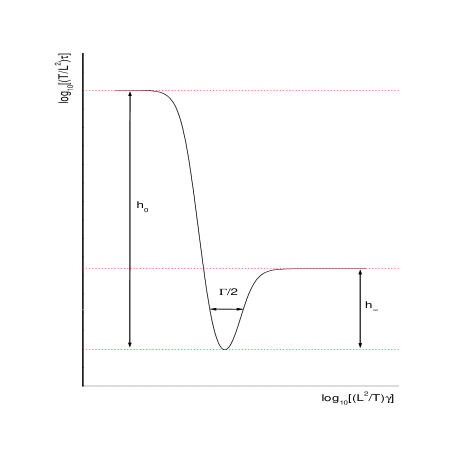
Figure 1: The resonant $\tau(\gamma)$ line and its asymptotes at low and high external noise frequencies.

In Section II, a brief statement of the “archetypal” resonance activation problem is presented. Section III discusses solutions to the problem posed for the arctan potential, pointing out special symmetry of this function that determines equality of the mean first passage time for convex and concave slopes approximating between the triangular, piecewise-linear and piecewise-constant forms of the potential. Numerical results are obtained and further analyzed to asses how sharp and persistent the resonant region of the mean first passage time can be as a function of the noise correlation time and steepness of the potential slope. We conclude with some final remarks in Section IV.

II Generic model system

We have considered an overdamped Brownian particle kra moving in a potential field between absorbing and reflecting boundaries in the presence of noise that modulates the barrier height. The evolution of a state variable $x(t)$ is described in terms of the Langevin equation

$$\frac{dx}{dt} = -V^{\prime}(x)+\sqrt{2T}\xi(t)+g(x)\eta(t)$$ (1)

$$= -V_{\pm}^{{}^{\prime}}(x)+\sqrt{2T}\xi(t).$$

Here $\xi(t)$ is a Gaussian process with zero mean and correlation $<\xi(t)\xi(s)>=\delta(t-s)$ (i.e. the Gaussian white noise arising from the heat bath of temperature $T$), $\eta(t)$ stands for a Markovian dichotomous (not necessarily symmetric) noise taking on one of two possible values $a_{\pm}$ and prime means differentiation over $x$. The correlation function of the dichotomous process satisfies $<\eta(t)\eta(t^{\prime})>=e^{-2\gamma|t-t^{\prime}|}{(a_{+}-a_{-})^{2}}/4$ where $\gamma$ stands for the flipping frequency of the barrier fluctuations (i.e. $\frac{1}{2\gamma}$ represents the characteristic correlation time of the dichotomous noise). Both noises are assumed to be statistically independent, i.e. $<\xi(t)\eta(s)>=0$. Equivalent to eq. (1) is a set of the Fokker-Planck equations describing evolution of the probability density of finding the particle at time $t$ at a position $x$, subject to the force $-V_{\pm}^{{}^{\prime}}(x)=-V^{\prime}(x)+a_{\pm}g(x)$

$$\partial_{t}{P}(x,a_{\pm},t) = \partial_{x}\left[V_{\pm}^{{}^{\prime}}(x)+T\partial_{x}\right]P(x,a_{\pm},t)$$ (2)

$$- \gamma P(x,a_{\pm},t)+\gamma P(x,a_{\mp},t)$$

In the above equations time has dimension of $[length]^{2}/energy$ due to a friction constant that has been “absorbed” in a time variable. We are assuming a reflecting boundary at $x=0$ and an absorbing boundary condition at $x=L$

$$P(L,a_{\pm},t)=0$$ (3)

$$\left[V_{\pm}^{{}^{\prime}}(x)+T\partial_{x}\right]P(x,a_{\pm},t)|_{x=0}=0.$$ (4)

The initial condition

$$P(x,a_{+},0)=P(x,a_{-},0)=\frac{1}{2}\delta(x)$$ (5)

expresses equal choice to start with any of the two configurations of the barrier. The quantity of interest is the mean first passage time

$$\tau = \int\limits_{0}^{\infty}dt\int\limits_{0}^{L}\left[P(x,a_{+},t)+P(x,a_{-},t)\right]dx$$ (6)

$$= \tau_{+}(0)+\tau_{-}(0)$$

with $\tau_{+}$ and $\tau_{-}$ being MFPT for $(+)$ and $(-)$ configurations, respectively. MFPTs $\tau_{+}$ and $\tau_{-}$ fulfill the set of backward Kolmogorov equations goel ; bork

$$-\frac{1}{2} = -\gamma\tau_{\pm}(x)+\gamma\tau_{\mp}(x)$$ (7)

$$- \frac{dV_{\pm}(x)}{dx}\frac{d\tau_{\pm}(x)}{dx}+T\frac{d^{2}\tau_{\pm}(x)}{dx^{2}}$$

with the boundary conditions (cf. eq. (3) and (4))

$$\tau_{\pm}^{{}^{\prime}}(x)|_{x=0}=0\qquad\tau_{\pm}(x)|_{x=L}=0$$ (8)

Although the solution of (7) is usually unique molenaar , a closed, “ready to use” analytical formula for $\tau$ can be obtained only for the simplest cases of the potentials (piecewise linear and piecewise constant). More complex cases, like even piecewise parabolic potential $V_{\pm}$ result in an intricate form of the solution to eq. (7). Other situations require either use of approximation schemes rei , perturbative approach iwa or direct numerical evaluation methods gam . In order to examine MFPT for various potentials, a modified program musn applying general shooting methods has been used with part of the mathematical software obtained from the Netlib library.

III Solution and Results

For $\gamma=0$ and $V_{+}(x)=V_{-}(x)=V(x)$, eq. (7) describes an overdamped Brownian particle moving in an external static potential (cf. eq. (1) with $\eta(t)\equiv 0$). In this situation a formula for the MFPT reads

$$\tau(0\to L) = \frac{1}{T}\int\limits_{0}^{L}d\eta\exp\left(\frac{V(\eta)}{T}\right)\int\limits_{0}^{\eta}\exp\left(-\frac{V(\xi)}{T}\right)d\xi$$ (9)

$$= \frac{1}{T}\int\limits_{0}^{L}\int\limits_{0}^{L}\exp\left(\frac{V(\eta)-V(\xi)}{T}\right)\theta(\eta-\xi)d\eta d\xi.$$

and does not depend on a constant part of a potential. Another non-trivial property in this case is equality of times

$$\tau(U,0\to L)=\tau(V,0\to L),$$ (10)

true for any two potentials $V(x)$, $U(x)$ that fulfill

$$U(x)=\mathcal{H}-V(L-x)$$ (11)

and are continuous functions mapping $[0,\;L]\to[0,\;\mathcal{H}]$. The above property can be simply proven after noticing that the difference

$$\tau(V,0\to L)-\tau(U,0\to L)=\int\limits_{0}^{L}\int\limits_{0}^{L}f(\eta,\xi)d\eta d\xi$$ (12)

with

$$f(\eta,\xi) = \left[\exp\left(\frac{V(\eta)-V(\xi)}{T}\right)-\exp\left(\frac{U(\eta)-U(\xi)}{T}\right)\right]$$ (13)

$$\times \frac{\theta(\eta-\xi)}{T}$$

vanishes for any points $(p,q)$ and $(p^{\prime},q^{\prime})$ such that $(p^{\prime},q^{\prime})$ is the image of $(p,q)$ in the reflection at the line $\eta=L-\xi$

$$f(p,q)=-f(p^{\prime},q^{\prime}).$$ (14)

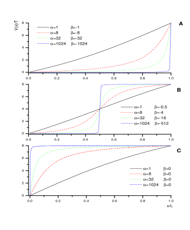
Figure 2: Potentials of arctan type for: A $\beta=-\alpha$, B $\beta=-\alpha/2$, C $\beta=0$.

To capture the features of the mean first passage time as a function of the shape of the barrier and characteristic correlation time of the barrier fluctuations, we have studied the Brownian diffusion problem in the arctan potential fluctuating randomly between two configurations $V_{+}(x)$ and $V_{-}(x)$

$$V_{\pm}(x) = \frac{H_{\pm}\mbox{arctan}(\alpha x/L+\beta)}{\mbox{arctan}(\alpha+\beta)-\mbox{arctan}(\beta)}$$ (15)

$$- \frac{H_{\pm}\mbox{arctan}(\beta)}{\mbox{arctan}(\alpha+\beta)-\mbox{arctan}(\beta)}.$$

Since switching between both configurations is modelled by a Markovian two-state process, the potential experienced by a particle remains in a given configuration for an exponentially distributed time, before flipping to the other state. The change in steepness and shift of the potential slope is controlled by parameters $\alpha$ and $\beta$. By using this particular form of the potential, we are able to modulate the steepness of the slope when holding the same, constant values of $V_{\pm}(x)$ at the bottom of the potential ($x=0,V_{\pm}(0)=0$) and at the top ($x=L,V_{\pm}(L)=H_{\pm}$) of the barrier (see Fig. 2). Moreover, as it is clearly seen from eq. (15), for $\beta=0$ and $\beta=-\alpha$, the potential satisfies the property eq. (11) with $\mathcal{H}=H_{\pm}$

$$V_{\pm}(x)|_{\beta=0}=H_{\pm}-V_{\pm}(L-x)|_{\beta=-\alpha}.$$ (16)

Thus, under the same type of barrier flipping process, the MFPT results are identical for the convex ($\beta=0$) and concave ($\beta=-\alpha$) potential slopes.

The standard numerical analysis molenaar ; rec of the MFPT has been performed for various forms of the potential eq. (15) with the slope changing accordingly to $\alpha=2^{i}$, $i=0,\dots,10$ and $\beta=-\alpha$ (Fig. 2 A), $\beta=-\alpha/2$ (Fig. 2 B) and $\beta=0$ (Fig. 2 C). The height of the potential barrier $H_{\pm}$ has been switching between either two symmetric values, $H_{\pm}=\pm 8T$, or “on” and “off” barrier positions, i.e. $H_{+}=8T,\;H_{-}=0$. Numerical analysis reestablishes discussed above equality of the MFPTs for potentials with $\beta=-\alpha$ and $\beta=0$. It means that for this set of parameters, the property eq. (10) observed for static potential, is also recovered for dichotomously fluctuating barriers

$$\tau(U,\gamma)=\tau(V,\gamma)$$ (17)

Therefore, graphical presentation of the results relates arbitrarily to the convex potentials only ($\beta=0$), having in mind that the same relationship $\tau(\gamma)$ is observed for the concave potentials with $\beta=-\alpha$ (cf. Fig. 2).

Generally with increasing slope of the barrier, resonant frequencies are shifted to higher values suggesting that more energy has to be pumped into the system in order to facilitate the escape of a Brownian particle over the fluctuating barrier. The minimal (resonant) values of $\tau$ increase with $\alpha$ for $V_{\pm}=\pm V$ potential and decrease for potentials switching between the “on-off” ($V_{+}=V,\;V_{-}=0$) positions, thus documenting a different character of resonant activation in these two cases, as discussed by Boguñá et al. boguna .

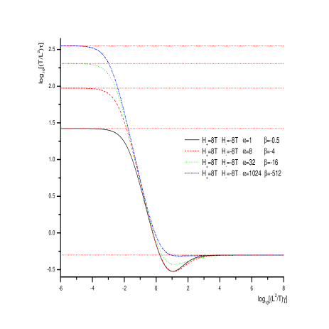
Figure 3: The $\tau(\gamma)$ as a function of barrier fluctuation rate for arctan potentials with $H_{+}=8T,\;H_{-}=-8T$, $\beta=-\alpha/2$.

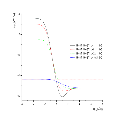
Figure 4: The $\tau(\gamma)$ as a function of barrier fluctuation rate for arctan potential with $H_{+}=8T,\;H_{-}=-8T$, $\beta=0$ ($\beta=-\alpha$).

For $V_{\pm}=\pm V$ barriers asymptotic values of MFPT at $\gamma\rightarrow\infty$ do not change with the steepness: they remain the same (Figs. 3, 4) and equal to $\frac{L^{2}}{2T}$, as predicted by analytical results for piecewise linear and piecewise constant potentials doe ; zucher ; boguna . However, they alter for the “on-off” potentials (cf. Figs. 5 and 6) displaying increase for $\beta=-\alpha/2$ and decrease for $\beta=0$ (same for concave potentials $\beta=-\alpha$). The resonant line (Fig. 1) of the $\tau(\gamma)$ dependence displays different features with zero and non-zero shift $\beta$. In particular, for $\beta=0$ the relative depths of minima measured from either the asymptotic $\tau$ value at $\gamma=0$ ($h_{0}$), or from the $\tau$ asymptote at $\gamma\rightarrow\infty$ ($h_{\infty}$) decrease with increasing $\alpha$ (cf. Figs. 4 and 6). For non-zero $\beta=-\alpha/2$ and both potentials, $V_{\pm}=\pm V$ or $V_{+}=V,\;V_{-}=0$, the relative depth $h_{0}$ increases with $\alpha$, as documented in Fig. 7 where the distance between the lines $\log_{10}[\tau(\gamma_{0})T/L^{2}]$ and $\log_{10}[\tau(\gamma_{min})T/L^{2}]$ is shown to increase with this parameter. At the same conditions, the depth of the resonant line $h_{\infty}$ measured from the asymptote at $\gamma\rightarrow\infty$ decreases for $V_{\pm}=\pm V$ potentials and increases for the “on-off” potentials $V_{+}=V,\;V_{-}=0$. These findings are summarized in Figs. 7 and 8 where logarithmic values of $\gamma_{min}$, $\tau(\gamma_{min})$, $\tau(\gamma_{0})$, $\tau(\gamma_{\infty})$ for the all arctan type potentials are plotted versus varying slope parameter $\alpha$.

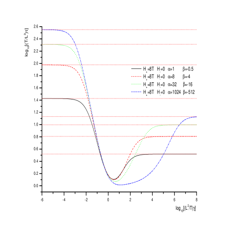
Figure 5: The $\tau(\gamma)$ as a function of barrier fluctuation rate for arctan potentials with $H_{+}=8T,\;H_{-}=0$, $\beta=-\alpha/2$.

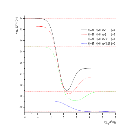
Figure 6: The $\tau(\gamma)$ as a function of barrier fluctuation rate for arctan potential with $H_{+}=8T,\;H_{-}=0$, $\beta=0$ ($\beta=-\alpha$).

Moreover, as can be easily seen in Figs. 5 and 6, the resonant width $\Gamma/2$ measured at $h_{\infty}/2$ (cf. Fig. 1) increases significantly for the “on-off” potentials with increasing value of the slope parameter $\alpha$. It is thus suggestive of an easier fine-tuning of the system to resonant conditions in this case by switching frequency of the barrier. The effect is also reproducible for $\beta=0$, although in this case the relative depth of MFPT minimum decreases, causing observable “flattening” of the resonant line.

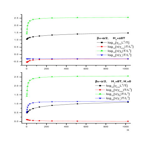
Figure 7: Location of minima, minimal and asymptotic values of the MFPT for arctan type potentials with $\beta=-\alpha/2$. Lines have been drawn to guide the eye.

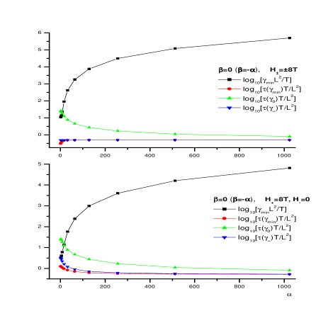
Figure 8: Location of minima, minimal and asymptotic values of the MFPT for arctan type potentials with $\beta=0$ ($\beta=-\alpha$). Lines have been drawn to guide the eye.

The functional dependence $\tau(\gamma)$ has a typical character in all cases discussed in this work. In agreement with theoretical considerations doe ; zucher ; pechukas ; rei ; reimann ; schmid ; hanggi , the asymptotic values $\tau(\gamma_{0})$ and $\tau(\gamma_{\infty})$ for large and small correlation times of the barrier noise are recovered with a minimum located in between those two. For all slopes of barriers this characteristic behavior of the MFPT remains similar although the weakening of the effect, i.e. shift of the resonant $\gamma_{min}$ to higher values and shallowing of the resonant line are observed with increasing steepness of the barrier. The effect of attenuation is stronger for $V_{\pm}=\pm V$ potentials with both, $\beta=-\alpha/2$ or $\beta=0$ ($\beta=-\alpha$). The resonant line flattens and slowly disappears with increasing $\alpha$ (i.e with increasing steepness of the barrier slope). The result is documented in Figs. 7 (upper panel) and 8, where the noticeable convergence between the values $\tau(\gamma_{min})$ and $\tau(\gamma_{\infty})$ is observed for $\alpha=1024$. Numerical estimates of MFPTs for the alternating potential ($V_{\pm}=\pm 8T$) yield $\tau(\gamma_{min})\approx 0.3$ and $\tau(\gamma_{\infty})\approx 0.5$ for $\alpha=8,\beta=-4$ leading to $h_{\infty}\approx 0.2$. This value drops by an order of magnitude to $h_{\infty}\approx 0.01$ for $\alpha=1024,\beta=-512$, that corresponds to by two-order of magnitude higher steepness of the slope estimated as the derivative of the potential at point $x=L/2$. Thus, the result suggests a fairly robust character of the resonant activation that disappears, but only for the limiting step-function potentials. An apparent persistence of the phenomenon for $V_{+}=8T,V_{-}=0$ and $\beta=-\alpha/2$ (Figs. 5 and 7, lower panel) is due to a different scenario of the barrier passage. In this particular case, an increasing $\alpha$ produces a wall at $x=L/2$ which has to be passed by a Brownian particle before being eventually absorbed at $x=L$. The particle experiences then a non-zero deterministic force at this point, only.

Potentials of the arctan type (eq. (15) and Fig. 2) produce barriers approximating between triangular and rectangular shapes mostly used for analytical studies of the resonant activation effect doe ; bier ; zucher ; boguna . Although the resonant phenomenon has been detected and analytically proven as a generic property in the case of dichotomously switching piecewise linear potentials doe ; zucher , it has been shown zucher not to occur in the case of piecewise constant potentials, when the Brownian particle escapes over either the small or the large barrier at all times. In consequence of the latter, barrier crossing events and barrier fluctuations are two independent stochastic processes zucher ; broeck ; reihan with the mean exit time decreasing monotonically from $\tau\approx\tau_{+}$ for $\gamma<\tau_{+}^{-1}$ to $\tau\approx\tau_{-}$ for $\gamma>\tau_{-}^{-1}$. The qualitative behavior of $\tau$ is then identical with the behavior of the exit time in so called kinetic models zucher ; broeck ; reimann ; pechukas ; gaveau which explicitly include the escapes over both high and low barriers at a rate $W_{\pm}=\exp(-H_{\pm}/T)$ and transitions between the two configurations of the potential. As it has been discussed by Bier and Astumian bier , the kinetic description assumes an instantaneous adiabatic adjustment and accordingly leads to the set of equations for the populations $\pi_{\pm}$ of particles that feel the potential $V_{\pm}$ and have not yet escaped over the barrier

$$\frac{d}{dt}\pi_{\pm}(t)=-W_{\pm}\pi_{\pm}-\gamma\pi_{\pm}+\gamma\pi_{\mp}$$ (18)

The decay of the survival probability $\pi(t)=\pi_{+}(t)+\pi_{-}(t)$ is then determined by an average MFPT

$$\tau\equiv\tilde{T}=-\int_{0}^{\infty}t\frac{d\pi(t)}{dt}dt=\frac{2\gamma+(W_{+}+W_{-})/2}{W_{+}W_{-}+(W_{+}+W_{-})\gamma}$$ (19)

which for slow barrier fluctuations ($\gamma=0$) approaches the average of the MFPT for the alternative configurations and in the fast fluctuation limit ($\gamma\rightarrow\infty$ but respecting $\gamma<<T_{s}^{-1}$, where $T_{s}^{-1}$ stands for the frequency of the escape attempts rei ; reimann ; reihan ) coincides with the reciprocal of the average rate over the fluctuating barrier. For fluctuating rectangular potentials with a barrier placed at $x=L/2$, the closed expressions for the mean escape time zucher for $\gamma=0$ and $\gamma\rightarrow\infty$ read

$$\tau(\gamma_{0})\frac{T}{L^{2}}=\frac{1}{2}\left[\frac{\tau_{+}+\tau_{-}}{2}\right],$$ (20)

$$\tau(\gamma_{\infty})\frac{T}{L^{2}}=\frac{1}{2}\left[1+\frac{\tau_{+}\tau_{-}-1}{2+\tau_{+}+\tau_{-}}\right]$$ (21)

and are perfectly reproduced in numerical MFPT studies in the $V_{\pm}=\pm V$ potential with parameters $\alpha=1024,\beta=-\alpha/2$ approximating a step-like function $\theta(x-L/2)$. However, in the case of the “on-off” potential $V_{+}=8T,V_{-}=0$ and the same set of parameters $\alpha$, $\beta$ numerical $\tau$ value for $\gamma\rightarrow\infty$ differs from the eq. (21) by four order of magnitude (cf. Figs. 7, 5) displaying a persistent resonant activation vanishing slowly at much steeper barriers which eventually reach the limit of an infinite tangent at $x=L/2$. Similarly to the former results zucher , in the limiting case of a piecewise constant potential, the mean exit time approaches $\tau\approx\tau_{+}$ for $\gamma<\tau_{+}^{-1}$ and $\tau\approx\tau_{-}$ for $\gamma>\tau_{-}^{-1}$ displaying an inverse proportionality to the rate of the barrier fluctuations for intermediate rates.

IV Summary

In the foregoing sections we have considered the thermally activated process that occurs in a system coupled to an external noise source. The external stochastic process is responsible for fluctuations of the potential barrier which has been modelled by an arctan function of varying slope. As expected based on previous theoretical studies doe ; rei , the phenomenon of resonant activation occurs typically in the system under broad circumstances of varying shape of the potential barrier and qualities of barrier fluctuations. In general, with increasing barrier steepness the resonance phenomenon becomes less “sharp” with the flat region of flipping frequencies around the resonant one. The time scale of the resonant activation process is fairly insensitive to the potential parameters except in the case of the “on-off” potentials, when broadening of the MFPT resonant line occurs suggesting most efficient tuning of the system to the resonance conditions.

- (1) W. Horsthemke and R. Lefever, Noise-Inducted Transitions. Theory and Applications in Physics, Chemistry, and Biology (Springer Verlag, Berlin, 1984).
- (2) N. G. van Kampen, Stochastic processes in physics and chemistry (North-Holland, Amsterdam, 1987).
- (3) Ch. R. Doering and J. C. Gadoua, Phys. Rev. Lett. 69, 2318 (1992).
- (4) J. Maddox, Nature 359, 771 (1992).
- (5) R. F. Fox and R. Roy, Phys. Rev. A 35, 1838 (1987).
- (6) K. Lee and W. Sung, Phys. Rev. E 60, 4681 (1999).
- (7) H. A. Kramers, Physica (Utrecht) 7, 284 (1940).
- (8) N. S. Goel and N. Richter-Dyn, Stochastics Models in Biology (Academic Press, San Diego, 1974).
- (9) J. Iwaniszewski, Phys. Rev. E 54, 3173 (1996).
- (10) P. Hängii, P. Talkner and M. Borkovec, Rev. Mod. Phys. 62, 251 (1990).
- (11) M. Boguñá et al., Phys. Rev. E 57, 3990 (1998).
- (12) R. M. M. Mattheij and J. Molenaar, Ordinary Differential Equations in Theory and Practice (John Wiley and Sons, Chichester, 1996).
- (13) P. Reimann, R. Bartussek and P. Hänggi, Chem. Phys. 235, 11 (1998).
- (14) L. Gammaitoni et al., Rev. Mod. Phys. 70, 223 (1998).
- (15) R. M. M. Mattheij, G. W. M. Staarink, MUS.F program for solving general two point boundary problems (http://www.netlib.org).
- (16) W. H. Press et al., Numerical Recipes in Fortran 77. The art of scientific computing (Cambridge University Press, Cambridge, 1992).
- (17) U. Zürcher and Ch. R. Doering, Phys. Rev. E 47, 3862 (1993).
- (18) P. Pechukas and P. Hänggi, Phys. Rev. Lett. 73, 2772 (1994).
- (19) P. Reimann, Phys. Rev. E 52, 1579 (1995).
- (20) G. J. Schmid, P. Reimann and P. Hänggi, J. Chem. Phys. 111, 3349 (1999).
- (21) P. Hänggi, Chem. Phys. 180, 157 (1994).
- (22) M. Bier and D. Astumian, Phys. Rev. Lett. 71, 1649 (1992).
- (23) C. Van den Broeck, Phys. Rev. E 47, 4579 (1993).
- (24) P. Reimann and P. Hänggi, in: L. Schimansky Geier, T. Pöschel (Eds.), Stochastic Dynamics, Lecture Notes in Physics, Vol. 484 (Springer Verlag, Berlin, 1997), p.127-139.
- (25) B. Gaveau and M. Moreau, Phys. Lett. 211A, 331 (1996).