Sustaining supercooled mixed phase via resonant oscillations of the order parameter

Abstract

We investigate the dynamics of a first order transition when the order parameter field undergoes resonant oscillations, driven by a periodically varying parameter of the free energy. This parameter could be a background oscillating field as in models of pre-heating after inflation. In the context of condensed matter systems, it could be temperature $T$, or pressure, external electric/magnetic field etc. We show that with suitable driving frequency and amplitude, the system remains in a type of mixed phase, without ever completing transition to the stable phase, even when the oscillating parameter of the free energy remains below the corresponding critical value (for example, with oscillating temperature, $T$ always remains below the critical temperature $T_{c}$). This phenomenon may have important implications. In cosmology, it will imply prolonged mixed phase in a first order transition due to coupling with background oscillating fields. In condensed matter systems, it will imply that using oscillating temperature (or, more appropriately, pressure waves) one may be able to sustain liquids in a mixed phase indefinitely at low temperatures, without making transition to the frozen phase.

Key words: Resonance, supercooling, phase transitions, preheating, inflation

I Introduction

Recently, it has been shown in ref.[1] that if an order parameter field undergoes resonant oscillations due to some parameter of the free energy, e.g. temperature (or pressure, background field etc.), being driven periodically, then a finite density of topological defects can arise even when the system never goes through the phase transition, and remains at temperatures much below the critical temperature $T_{c}$. Also, the spatial distribution of order parameter at late times resembled more like a system undergoing phase transition, rather than the ordered phase at low temperatures. It was speculated in [1] that this phase may have interesting properties. In the present paper we address this issue for the case of a first order transition. We will briefly comment on the case of a second order transition (which was the case in ref.[1]), a detailed discussion of that case is postponed for a future publication.

Consider a system, supercooled, and trapped in the metastable high temperature phase, as denoted by the free energy plot (solid curve) in Fig.1. If the system is left in this stage, critical bubbles of the low temperature stable phase will nucleate via thermal fluctuations, will grow, coalesce, and convert the entire system to the stable phase. We will study the dynamics of this transition, using numerical simulation, when some parameter of the free energy is undergoing periodic variations, leading to periodic changes in the shape of the free energy plot as indicated by dashed curves in Fig.1. This will drive the order parameter field away from the stable phase, inducing field oscillations. Occasionally, localized resonances will force the field to go across the barrier, all the way up to the metastable vacuum. Such a region will shrink again, while more regions bounce to the metastable phase.

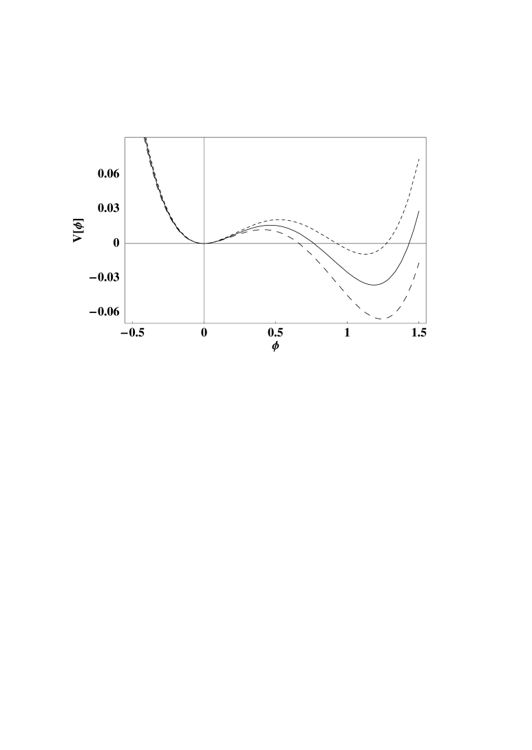
FIG. 1.: The plot of free energy undergoing periodic variations, with $T$ remaining below $T_{c}$. Order parameter $\phi$ will be frequently driven via localized resonant oscillations, over the barrier into the metastable phase. Note that we use suitably scaled, dimensionless variables as explained in Eq.(1).

As we will see below, the resulting distribution of the order parameter is similar to that corresponding to the mixed phase which (at low temperatures) exists only for short time during the usual first order phase transitions. Here this phase is sustained for as long as the free energy keeps varying periodically.

The physical implications of the possibility of achieving such a phase can be important. For example, in the context of cosmology, with oscillating parameter being a background field (as in models of pre-heating after inflation), this will mean a prolonged existence of the mixed phase during a first order phase transition, thereby affecting the final reheating temperature. In the context of condensed matter systems, if one could achieve such a phase for water (or any liquid), then at temperatures much below the freezing temperature, with the system subjected to periodically varying temperature, or more appropriately, pressure (density waves with suitable frequency and amplitude), microscopic ice crystals may form, but they will not be able to grow bigger. The whole system will remain in a mixed phase of microscopic ice crystals continuously forming, and decaying, but never completing the transition to the frozen phase. Crucial point is that all this can be achieved while the temperature of the system remains below the critical temperature. In general, for any first order transition, one may be able to indefinitely sustain mixed phase in supercooled (or superheated) state in this manner. In this context we mention that it has been discussed in the literature that the structure of supercooled water is very similar to the known structure of high density amorphous ice [2]. There have also been several studies where systems in a non-equilibrium state approach quasi-stationary phases with very large relaxation time scales. For example, recent studies have discussed similarities between the dynamics of granular materials and glassy materials under the influence of external periodic influence (see, e.g. [3]). The existence of (quasi) stationary phases in such systems [3, 4] (for relevant time scales) may thus appear similar to what we have discussed here, though the underlying physics is quite different.

Another important issue which has been discussed in earlier studies of non-equilibrium systems with slow dynamics relates to the notion of an effective temperature [5] (see, also, refs.[3, 4]). It has been discussed that the fluctuation-dissipation relation can be generalized for such systems with an effective temperature which acts like the thermodynamic temperature in the sense that it controls the direction of heat flow and acts as a criterion for thermalization. In the context of our model also one would like to know if such an effective temperature can be defined and whether that effective temperature is significantly higher than the temperature used in the expression for the free energy of the system. Thus when we make statements like the temperature of the system being much below the critical temperature, we are ignoring, for the purpose of the present work, these issues relating to the effective temperature etc. for the non-equilibrium system at hand. We hope to address these issues in a future work where we will also investigate the issue of appropriate meaning of re-heat temperature in models of pre-heating after inflation.

The paper is organized in the following manner. In section II we describe our model, and discuss basic physics involved. Section III presents results of our numerical simulations. Conclusions and discussions are presented in section IV.

II Description of the system

We will discuss the dynamics of a system in 2+1 dimensions, described by the following free energy (effective potential), which is expressed in terms of scaled, dimensionless variables for simplicity of presentation [1].

$$V(\phi)=\frac{1}{4}\phi^{2}(\phi-1)^{2}-{\epsilon\over 2}\phi^{3}+{1\over 4}T(t)\phi^{2},$$ (1)

with $T(t)$ being the instantaneous temperature of the system, which is taken to be spatially uniform. We take the time dependence of the temperature to be,

$$T(t)=T_{0}+T_{a}\sin(\omega t).$$ (2)

Above, $\phi$ is a scalar order parameter, and we take $\epsilon=0.1$. From Eq.(1), we get the critical temperature $T_{c}=(1+\epsilon)^{2}-1=0.21$. We discuss the 2+1 dimensional case due to computer limitations. We expect similar results for 3+1 dimensions, as the basic physics of resonant field oscillations remains the same. We hope to discuss the 3+1 dimensional case in a future presentation. We emphasize that the crucial physics of our model resides in the time dependence of the free energy. We have characterized this in terms of a time dependent temperature. One could also do this by periodically varying some other parameter such as pressure, which may be experimentally more feasible, or possibly, even a time-dependent external electric or magnetic field (say, for liquid crystals). In the context of cosmology this time dependence can be achieved by coupling to a background oscillating field, as discussed below.

We use the following equations for field evolution.

$$\partial^{2}\phi/\partial t^{2}+\eta\partial\phi/\partial t-\bigtriangledown^{2}\phi+V^{\prime}(\phi)=0.$$ (3)

Here $\eta$ is the dissipation coefficient. We have included the term with second order time derivative, (the inertial term [6]), since the short time scale dynamics of $\phi$ is of crucial importance here. We do not include a noise term in Eq.(3). The basic physics we discuss does not depend on noise. Also, as discussed above, time dependence of the free energy could arise from some other source, with temperature kept low to suppress any thermal fluctuations (though, we again mention that we are ignoring here the possibility of defining an effective temperature [5]). In any case, noise due to thermal fluctuations should further help in sustaining the mixed phase (e.g. in ref.[7] it is shown that presence of noise enhances the resonant oscillations of the field, leading to enhanced defect production). In a future work we will study the detailed effects of noise in our model, especially in the overdamped limit, and also explore connections with the well studied phenomenon of stochastic resonance in condensed matter systems [8].

As we indicated above, Eq.(3) with oscillatory T(t) is similar to the equation for an oscillating inflaton field coupled to another scalar field in the models of post-inflationary reheating in the early universe[9, 10], with $T(t)$ playing the role of the inflaton field. The results in the present paper (as well as in ref.[1]), therefore, have similarities with those models, though there are crucial differences. For example, it has been suggested in [10] that the completion of the transition after inflation may get delayed due to parametric resonance instabilities. Ref.[10] discusses the case of a homogeneous order parameter field coupled to a background oscillating inflaton field, and it is shown that due to parametric resonance the (uniform) order parameter keeps flipping between the stable minima and the metastable one. As we will see below, the actual physics of resonating order parameter for a first order transition case is much more complex. For example, field in localized regions is resonantly driven to the metastable vacuum where it can shrink down due to high free energy cost instead of being resonantly driven back to the stable vacuum. For the universe, the transition is eventually completed to the low temperature phase, as the oscillating inflaton field decays. In contrast, in the condensed matter case, where the periodic driving of temperature/pressure can be maintained indefinitely, the continued localized hopping of $\phi$ between the metastable vacuum and the stable vacuum keeps the system indefinitely in a mixed phase.

III Results

We first discuss the situation with fixed $T=T_{0}=0.1$. For $T<T_{c}$, $V(\phi)$ has a local minimum at $\phi=0$ (metastable phase),while the true minima (stable phase) occurs at $\phi\equiv\phi_{s}$ where,

$$\phi_{s}=\frac{1}{4}[3(\epsilon+1)+\sqrt{9(\epsilon+1)^{2}-8(T(t)+1)}~{}~{}]$$ (4)

With $T=0.1$ we get $\phi_{s}=1.186$. The plot of $V(\phi)$ at $T=0.1$ is shown by the solid curve in Fig.1. We start with a region of space trapped in the metastable phase with $\phi=0$. At finite temperature, the phase transition takes place by nucleation of bubbles of stable phase via thermal fluctuations [11, 12]. (For very low, or zero temperature, one may need to consider quantum nucleation of bubbles.) We simulate the nucleation of these bubbles using techniques developed in [11]. Bubbles nucleate with (slightly larger than) critical size and expand, ultimately filling up the space. The critical bubble profile is obtained by solving the following field equation [11, 12]

$${d^{2}\phi\over dr^{2}}+{1\over r}{d\phi\over dr}-V^{\prime}(\phi)=0,$$ (5)

subject to the boundary conditions $\phi(\infty)=0$ and $d\phi/dr=0$ at $r=0$; where $r$ is the radial coordinate. Note that, for our present discussion, the only relevant thing is the late time field configuration, and its evolution. The bubble configuration obtained by above method provides an adequate starting configuration here. Bubble nucleation is achieved by replacing a region of the metastable phase (false vacuum) by the bubble profile, which is suitably truncated with due care of smoothness of the configuration on the lattice. Subsequent evolution of the initial field configuration is governed by Eq.(3) with ${\dot{\phi}}=0$ at $t=0$.

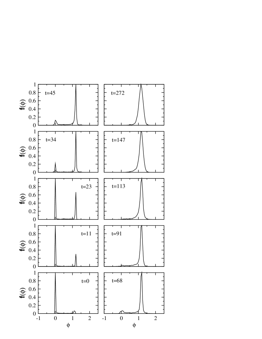
FIG. 2.: The plots of the distribution $f(\phi)$ vs. $\phi$ for the phase transition process simulated via bubble nucleation with $\omega=0$ in Eq.(2). Plots showing presence of two peaks correspond to the mixed phase. At late stages, this mixed phase completely disappears, and one gets a pronounced peak at the stable value of $\phi=\phi_{s}$ indicating the completion of the phase transition.

Nucleation of several bubbles is achieved by randomly choosing the location of the center of each bubble with some specified probability per unit volume [11]. (For simplicity we nucleate all the bubbles at the initial time. Time depended nucleation will not affect the phenomenon discussed in this paper.) If there is an overlap with a previously nucleated bubble, then nucleation of the new bubble is skipped. The simulation is done on a square lattice with periodic boundary condition, i.e on a torus. The field configuration is evolved by using a discretized version of Eq.(3), using a second order, staggered, leapfrog algorithm. The size of the lattice taken is $900\times 900$ with $\Delta x=0.16$ and $\Delta t\simeq 0.0075$. Simulations were carried out on HP workstations at the Institute of Physics, Bhubaneswar. As we are interested in the nature of the mixed phase, we present our results in terms of plots of the fraction $f(\phi_{0})$ representing the fractional volume of the region (calculated by counting the number of lattice sites) where $\phi$ lies between $\phi_{0}$ and $\phi_{0}+\Delta\phi$, for a suitable choice of $\Delta\phi$. We use $\Delta\phi=0.05\simeq 0.042\phi_{s}$. Here $\phi_{s}\simeq 1.186$ for $T=0.1$. The plots are normalized by taking the largest value of $f(\phi)=1$ for the given plot.

Fig.2 shows the results of the simulation (with $\eta=0$). The plot at $t=0$ shows the initial $f(\phi)$ which has a sharp peak at the background metastable phase, $\phi=0$, and a smaller peak at $\phi=\phi_{s}\simeq 1.19$ corresponding to stable phase inside the nucleated bubbles. (In each of the cases discussed here and below, 3 bubbles were nucleated.) The relative heights of the two peaks changes as the bubbles expand. At sufficiently late times, the only peak remains at $\phi=\phi_{s}$, indicating the completion of the phase transition to the stable phase. Plot of $f(\phi)$ remains essentially unchanged for all subsequent times. Bubble wall coalescence leads to $\phi$ oscillations which persist, due to absence of dissipation, contributing to the width of the peak at $\phi_{s}$ at late times. The nature of the plots will remain the same in the case even with non-zero $\eta$, which only affects the bubble wall velocities, and damping of $\phi$ oscillations (leading to sharper peak at late times).

We now repeat this simulation with non-zero value of $\omega$ in Eq.(2). We use $T_{0}=0.1$ and $T_{a}=0.08$, and $\omega=0.78$. With $T_{c}=0.21$, we note that the maximum value of $T$ remains below $0.9T_{c}$, while the average $T$ is below $0.5T_{c}$. Upper and lower dashed curves in Fig.1 show the plots of $V(\phi)$ at $T=T_{0}+T_{a}$, and $T=T_{0}-T_{a}$, respectively. We use $V(\phi)$ in Eq.(5) with $T=T_{0}+T_{a}=0.18$ for calculating the bubble profile. This is to make sure that the bubbles continue to expand during the oscillation of $T$. Size of the critical bubble obtained from Eq.(5) is about 24.1. $T$ in Eq.(1) is taken to be spatially uniform, with its periodic variation given by Eq.(2). The choice of frequency $\omega$ was guided by the range of frequency required to induce resonance for the case of spatially uniform field evolved by Eq.(3) (as in ref.[1]). (See,also, in this context, the discussion relating to the parametric resonance in ref.[13].) We find that resonance happens when $\omega$ lies in a certain range. We are assuming that for the relevant range of $\omega$ here, the system can be considered in quasi-equilibrium so that the use of time dependent $V$ makes sense. This frequency range, for which resonant oscillations of $\phi$ occurs, depends on $T_{0}$ as well as on $T_{a}$, with the range becoming larger as $T_{0}$ approaches $T_{c}$. Basically, the value of $\omega$ should be such that $\phi$ oscillations should be affected significantly by the changes in the shape of $V(\phi)$ (as argued in ref.[1]). Thus one expects that $\omega$ should be roughly of the same order as the natural frequency of oscillation of the order parameter near the stable minimum of the free energy. With the above values of $T_{0}$ and $T_{a}$, the range of $\omega$ is found to be between 0.68 and 0.98. We present results for $\omega=0.78$.

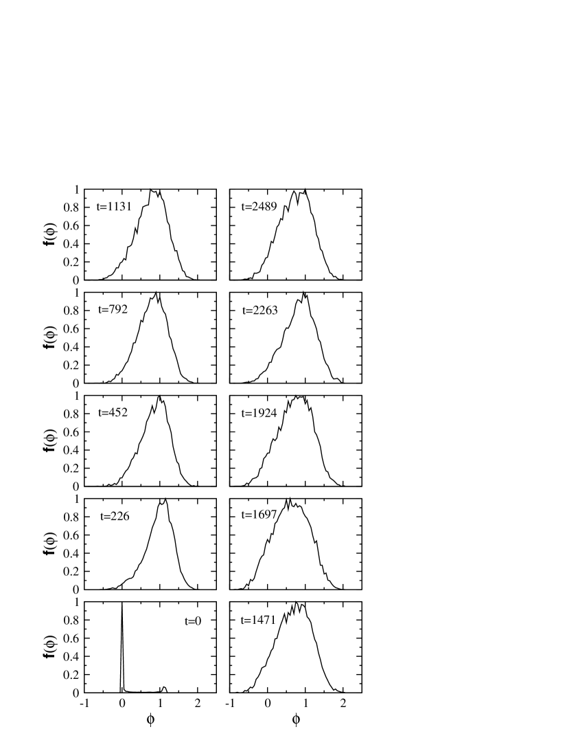
FIG. 3.: The plots of the distribution $f(\phi)$ vs. $\phi$ for the case with $\omega=0.78$. Plots for late times show significant support at small values of $\phi$. $f(\phi=0)$ keeps fluctuating between 20 % to 50 % at all late times, clearly demonstrating that the transition never gets completed to the stable phase.

As discussed above, this periodic variation in $V(\phi)$ drives $\phi$ periodically and leads to frequent resonances [1]. Occasionally, $\phi$ in a small region is able to get resonantly driven all the way over the barrier. Thus, in the regions where $\phi\simeq\phi_{s}$, occasionally a small patch of metastable value $\phi=0$ forms. This patch is energetically unstable, so it shrinks. Or, it could also oscillate to the stable phase. Crucial point here is that even as bubbles all coalesce, $\phi$ still keeps flipping over the barrier to the metastable value $\phi=0$ keeping the system in a mixed phase. This will keep happening as long as the system is periodically driven with appropriate value of $\omega$ in Eq.(2). We mention that even the largest patch we find, where $\phi$ flips over the barrier to the metastable value, has size much smaller than the critical bubble size, otherwise one could nucleate stable phase bubbles there.

Fig.3 shows the evolution of the distribution $f(\phi)$ for this case. The plot at $t=0$ is the same as in Fig.2. However, now, as bubbles coalesce, instead of getting a more and more pronounced peak only at the stable value of $\phi=\phi_{s}$, we are getting a very broad distribution of $f(\phi)$. Note, in particular, that $f(\phi)$ at the metastable value $\phi=0$ is never zero, in complete contrast to the situation in Fig.2.

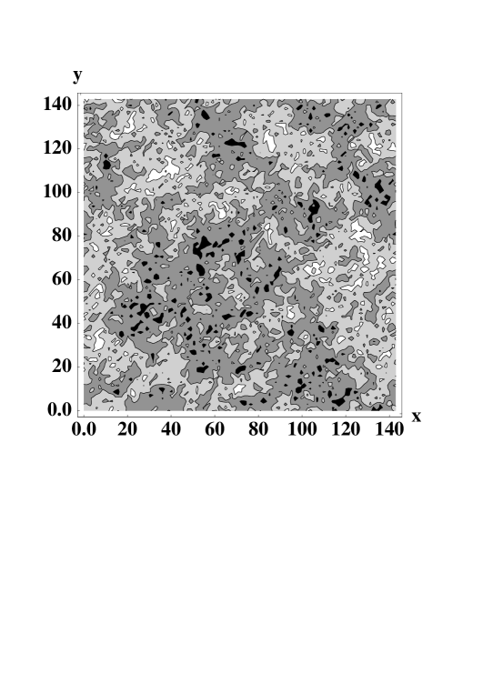
FIG. 4.: Contour plot of spatial distribution of $\phi$ at $t=1697$. White regions correspond to $\phi=0$, while black regions correspond to the largest value of $\phi$ at this stage. Mixing of dark and light regions is a clear evidence of the existence of the mixed phase.

In fact the ratio of the volume where $\phi=0$, to the volume where $\phi$ is near the oscillating stable vacuum (where $f(\phi)\simeq 1$ with our normalization) keeps fluctuating between about 20% to almost 50 % at all late times. (Non-zero values of $f(\phi)$ at negative $\phi$ result due to oscillations of $\phi$ about $\phi=0$.) This is the direct evidence that the system never completes the phase transition to the stable phase, and remains in the mixed phase indefinitely. This is further evidenced by the contour plot of $\phi$ in Fig.4. Here, shading represents the value of $\phi$, with white region corresponding to the smallest value of $\phi$ (which is negative due to $\phi$ oscillations about $\phi=0$), while black region corresponding to the largest value of $\phi$ in a given plot. Existence of mixed phase is clear by the mixing of dark and light regions. Another important thing to note is that neither white, nor black regions occur in large sizes (compared to the critical bubble radius $\simeq 24.1$ as mentioned above). Further, value of $\phi$ keeps fluctuating rapidly at any given point, as we will see below. Thus there are no regions where even in an approximate sense phase transition can be said to be completed to the stable phase. Similar features can be seen in Fig.5 which shows 3-dimensional plot of $\phi$ in a small portion of the lattice. Fluctuations in $\phi$ are seen to fill up the entire physical region.

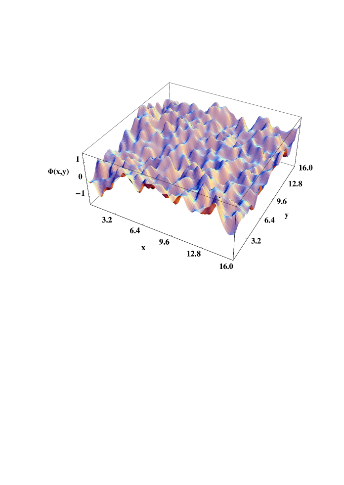
FIG. 5.: 3-dimensional plot of $\phi$ at $t=2602$ for a small portion of the lattice.

To better understand the resonantly driven dynamics of field here, we show, in Fig.6, plot of $\phi(x)$ at an arbitrary fixed point for a small time duration. While oscillating, $\phi$ bounces back at some point $\phi>\phi_{s}$ ($\simeq$ 1.2 for the $V(\phi)$ shown by the solid plot in Fig.1), and towards the metastable minimum, at some negative value of $\phi$. That is, resonant oscillations drive field from one minimum of $V(\phi)$ to the other. In between, $\phi$ executes oscillations about $\phi=0$, and about the stable vacuum. The detailed dynamics of $\phi(x)$ at a given point is much more complex than simple oscillations about the two minima (and resonant driving in between the two), due to the effect of density waves coming from other regions, shrinking of regions of metastable vacuum etc. (As we mentioned above, such features, which strongly affect the nature of resulting mixed phase, could not be seen in ref.[10] where order parameter was taken to be uniform). Still, the plot in Fig.6 shows that the qualitative aspects of the field dynamics are dominated by oscillatory motions, and not by some random noise (which would be the case for thermal fluctuation dominated dynamics). This is consistent with the physical picture outlined above that the system is in a complete non-equilibrium state, being continuously driven by the periodically varying temperature in Eq.(1).

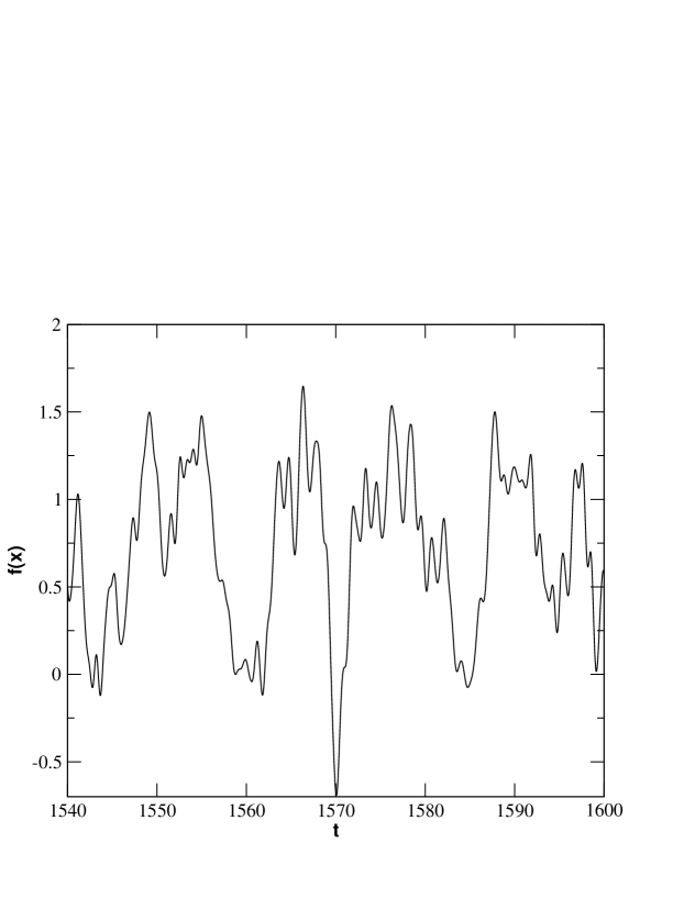
FIG. 6.: Evolution of $\phi(x)$ at an arbitrary, fixed point. The detailed dynamics of $\phi(x)$ at a given point is more complicated than simple oscillations about the two minima (and resonant driving in between the two), due to the effect of density waves coming from other regions, etc.

We now consider the case of non-zero dissipation. As expected, for large values of $\eta$, $\phi$ oscillations damp fast, suppressing resonant oscillations (as found in ref. [1]). For small $\eta$, as in Fig.7, oscillations are somewhat suppressed, but the mixed phase is still sustained. In Fig.7 we give plots of $f(\phi)$ for the case with $\eta=0.01$. As mentioned above, in view of results in ref.[7], we expect that inclusion of noise term in Eq.(3) will lead to enhanced resonances (possibly even in the overdamped limit). Note that the distribution of $f(\phi)$ for the mixed phase in Fig.3,7 is very different from the mixed phase plots in Fig.2. It will be interesting to explore if there are essential physical differences between these two types of mixed phases. It is possible that with the inclusion of thermal fluctuations this difference may reduce.

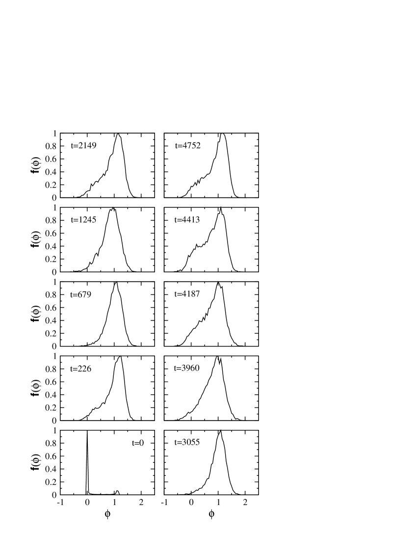
FIG. 7.: The plots of the distribution $f(\phi)$ vs. $\phi$ for the case with $\eta=0.01$. Even here, we find that plots for late times show significant support at small values of $\phi$. $f(\phi=0)$ keeps fluctuating between 5 % to 20 % at all late times.

It is important to mention here that the existence of a local minimum (at $\phi=0$ in Eq.(1)) is crucial in getting significant support for $f(\phi)$ near $\phi=0$. When $\phi$ is resonantly driven over the barrier to that local minimum, it may get trapped there, oscillating about $\phi=0$, until the region shrinks away (as mentioned above, this region is always too small to nucleate another bubble there). When we use a free energy similar to that in ref.[1] (appropriate for a second order transition), we find that distribution of $f(\phi)$ still broadens at $\phi_{s}$, but it does not develop significant support at $\phi=0$. (That is the situation with complex $\phi$. If we take real $\phi$ with the $V$ in ref.[1], then significant volume fraction with $\phi$ = 0 arises due to regular production and shrinking of extended domain wall defects.) However, we emphasize that even in the case of ref.[1], the distribution of $\phi$ at late times resembles the situation of an equilibrium system which is close to the transition point, even when the temperature remains much below the critical values. (We make this statement in a loose sense, basically focusing on qualitative features of domain structure and fluctuations). The physical properties of that system will therefore be completely different from the one expected from the system at the value of the temperature used in $V$, just as demonstrated here for the case of first order transition.

IV Discussion and Conclusions

Our results show a very interesting possibility, and at the same time raise many questions. The physical nature of such a system looks very different from the system at the temperature used in $V$ in Eq.(1). Though we are discussing the situation of non-equilibrium, the system seems to reach a state of quasi-equilibrium, or, more appropriately, a stationary state, where its average properties do not fluctuate too much, such as the distribution of fraction $f(\phi)$ in Figs.3,7. We mention here again that there may be a possibility of defining some sort of effective temperature here, following the discussions in the literature [5]. It will then be interesting to determine how the properties of the system we observe relate to the expected properties of the system at that effective temperature.

Also, as we discussed earlier, though we have characterized the periodically varying term in $V(\phi)$ in Eq.(1) in terms of a periodically varying temperature, it could be achieved in various different ways. For example, in cosmology, coupling to a background oscillating inflaton field will give rise to required driving of the order parameter field [9, 10]. In many condensed matter systems (e.g. liquids) periodic variation of pressure may be a better choice as that can easily be induced by density waves. (From that point of view it will be interesting to consider periodic temporal as well as spatial variations of the parameter in $V(\phi)$.) For some systems, such as liquid crystals, periodically varying external fields (electromagnetic field) may be more suitable. We emphasize that, though actual numbers (e.g. fraction of the system in the metastable phase etc.) will vary from one system to other, (and from $2+1$ dimensional case discussed here to the $3+1$ dimensional case), the basic physics of the phenomenon we have discussed here appears very robust. A rapidly oscillating free energy, due to periodic variation of its parameter(s), will in general be expected to lead to resonant oscillations of the order parameter, with appropriate frequency and amplitude of the oscillating parameter. This will lead to periodic, localized creations of regions with metastable phase, even when the temperature (and other parameters) of the system always remain much below the transition point (or above it, for the case of superheating). Resulting phase is similar to the mixed phase which can be sustained for as long as the system is periodically driven.

For cosmology, this phenomenon will imply an extended period of mixed phase, until the background oscillating inflaton field decays. This will affect the value of final reheat temperature after inflation. In the context of condensed matter systems this possibility of indefinitely sustaining mixed phase of systems at temperatures below the critical temperature can have very important implications, especially for supercooling liquids. It is tempting to speculate that if such a possibility can be realized for water, then it would imply that supercooling organisms may be possible (when subjected to, say, pressure waves of suitable frequency and amplitude) without freezing, as large ice crystals will never form. (Note, again, we are ignoring here the issues relating to the effective temperature [5] which could be defined for the non-equilibrium system at hand. It is possible that such an effective temperature may not be as low as the temperature which is used in the expression of the free energy in Eq.(1). We hope to investigate these issues in a future work.) As mentioned above, the appropriate range of $\omega$, for the phenomenon we discuss, will be expected to be of the order of the natural frequency of oscillation of the order parameter near the stable minimum of the free energy of the specific system being considered. Thus, it should be possible to experimentally verify this possibility in condensed matter systems by subjecting liquids (water) to density waves using a varying range of frequency and amplitude, while supercooling below $T_{c}$.

ACKNOWLEDGEMENTS

We are very thankful to A.P. Balachandran, Sanatan Digal, Biswanath Layek, Rashmita Sahu, and Supratim Sengupta for useful discussions and comments. AMS would like to acknowledge the hospitality of the Physics Dept. Univ. of California, Santa Barbara while the paper was being written. His work at UCSB was supported by NSF Grant No. PHY-0098395.

REFERENCES

- [1] S. Digal, R. Ray, S. Sengupta, and A.M. Srivastava, Phys. Rev. Lett. 84, 826 (2000).
- [2] F.W. Starr, M.C. Bellissent-Funel, and H.E. Stanley, Phys. Rev. E 60, 1084 (1999).
- [3] L. Berthier, L.F. Cugliandolo, and J.L. Iguain, Phys. Rev. E 63, 051302 (2001).
- [4] L.F. Cugliandolo and J. Kurchan, Phys. Rev. Lett. 71, 173 (1993).
- [5] P.C. Hohenberg and B.I. Shraiman, Physica D 37, 109 (1989); M. Caponeri and S. Ciliberto, Physics D 58, 365 (1992); L.F. Cugliandolo, J. Kurchan, and L. Peliti, Phys. Rev. E55, 3898 (1997).
- [6] Recent developments in nonequilibrium thermodynamics, Lecture Notes in Physics, Vol. 199, Edited by, J.C. Vazquez, D. Jou, and G. Lebon, (Springer-Verlag, Berlin, 1984).
- [7] R. Ray and S. Sengupta, Phys. Rev. D 65, 063521 (2002).
- [8] L. Gammaitoni et al, Rev. Mod. Phys. 70, 223 (1998); see also, R. Benzi, A. Sutera, and A. Vulpiani, J. Phys. A 18, 2239 (1985); F. Marchesoni, L. Gammaitoni, and A.R. Bulsara, Phys. Rev. Lett. 76, 2609 (1996); see also, G. Korniss, P.A. Rikvold, and M.A. Novotny, cond-mat/0207275.
- [9] J.H. Traschen and R.H. Brandenberger, Phys. Rev. D 42, 2491 (1990); L. Kofman, A. Linde, and A.A. Starobinsky, Phys. Rev. Lett. 73 3195 (1994); V. Zanchin, A. Maia, Jr., W. Craig, and R. Brandenberger, Phys. Rev. D 60, 023505 (1999).
- [10] J.M. Cornwall and A. Kusenko, Phys. Rev. D 61, 103510 (2000).
- [11] A.M. Srivastava, Phys. Rev. D 45, R3304 (1985); S. Chakravarty and A.M. Srivastava, Nucl. Phys. B 406, 795 (1993).
- [12] A.D. Linde, Phys. Lett. B 100, 37 (1981); M.B. Voloshin, I.Yu. Kobzarev, and L.B. Okun, Sov. J. Nucl. Phys. 20, 644 (1975); S. Coleman, Phys. Rev. D 15, 2929 (1977).
- [13] L.D. Landau and E.M. Lifshitz, Mechanics, (Pergamon Press, 1969).