Two-component Bose-Einstein Condensates with Large Number of Vortices

Erich J. Mueller[1] and Tin-Lun Ho[2] Department of Physics, The Ohio State University, Columbus, Ohio 43210
Abstract

We consider the condensate wavefunction of a rapidly rotating two-component Bose gas with an equal number of particles in each component. If the interactions between like and unlike species are very similar (as occurs for two hyperfine states of 87Rb or 23Na) we find that the two components contain identical rectangular vortex lattices, where the unit cell has an aspect ratio of $\sqrt{3}$, and one lattice is displaced to the center of the unit cell of the other. Our results are based on an exact evaluation of the vortex lattice energy in the large angular momentum (or quantum Hall) regime.

pacs:
03.75.Fi,47.32.Cc

Experiments on rotating Bose gases have progressed rapidly in the last two years. Soon after the pioneer work at JILA [3] and ENS [4], the MIT group created a vortex lattice with as many as 160 vortices[5]. Recently, the JILA group has invented an ingenious method to increase the angular momentum of a condensate by performing evaporative cooling on a rotating normal cloud[6]. In this process, the system spins faster and faster as it is cooled, while remaining close to equilibrium. With such rapid progress, one expects that equilibrium Bose gases with even larger angular momenta may be produced in the near future.

At present, most experiments on vortex lattices are performed in single component Bose systems. It is natural to ask what happens in two-component Bose gases, such as those made up of two hyperfine spin states of the same atom. The vortex lattices in such systems are bound to be more intricate than those in single component condensates, as the vortices in different components can move relative to one another to minimize the energy. The purpose of this paper is to study the vortex lattices of two-component systems with large number of vortices, in what we call the “mean-field quantum Hall regime”. This is the regime where mean field theory remains valid so that each component (labeled by an index “$i$”, $i=1,2$) is characterized by a condensate wavefunction $\Psi_{i}$; yet the angular momentum of the system is so high that $\Psi_{i}$ is made up of the orbitals in the lowest Landau level in the plane perpendicular to the rotation axis. It has been shown recently[7] that this regime will emerge in a three dimensional Bose gas at sufficiently high angular momenta [8]. We focus on this regime because the wavefunction in this limit acquires an analytic structure which allows exact evaluation of the energy of a vortex lattice. As a result, it is possible to scan through a wide range of lattice structures which would be impractical for numerical calculations because of the time and the accuracy required. Although not directly applicable to current experiments on vortex lattices (which are performed at lower angular momenta), the physics of the mean field quantum Hall regime is still quite relevant as the vortex lattices in these two regimes are connected continuously to each other.

One special feature of the majority of two-component gases so far studied, (notably mixtures of hyperfine states of 87Rb [9] in magnetic traps, or 23Na [10] in optical traps) is that the interactions between like species (denoted $g_{1}$ and $g_{2}$) and unlike species (denoted $g_{12}$) are very similar, within a few percent of each other. Thus, if there are an equal number of bosons in each component, and if the trapping potentials of the two components are made identical, then the two components will be the same size and contain the same density of vortices. In this case, one expects that each component will contain identical vortex lattices, with one lattice displaced relative to the other. While we are mainly interested in the experimentally relevant cases, where $g_{1}\sim g_{2}\sim g_{12}$, considerable insight is gained by studying vortex lattices as a function of the interactions. Considering the case $g_{1}\sim g_{2}\neq g_{12}$, we find a wide range of vortex lattice structures as the parameter $\alpha=g_{12}/\sqrt{g_{1}g_{2}}$ is varied. The vortex lattice has a fixed structure over certain intervals of $\alpha$, while it varies continuously in others. The structure near the isotropic point $g_{1}=g_{2}=g_{12}$ consists of identical rectangular lattices in both components, with one displaced to the center of the unit cell of the other. The aspect ratio of the unit cell changes with $\alpha$, and is $\sqrt{3}$ when $\alpha=1$.

The mean-field quantum Hall regime: The condensate wavefunctions $\Psi_{1}$ and $\Psi_{2}$ of a two-component rotating Bose gas are determined by minimizing the grand potential $K=E-\Omega L_{z}-\mu_{1}N_{1}-\mu_{2}N_{2}$, where $E$ is the energy of the system, $\Omega$ is the rotational frequency, $L_{z}$ is the angular momentum along $z$, and $\mu_{i}$ ($i=1,2$) are the chemical potentials fixing the number of bosons $N_{1}$ and $N_{2}$ in each component. For simplicity, we assume identical trapping potentials for each component. We consider a cigar shaped trap with the symmetry axis $z$ coinciding with the axis of rotation. As discuss in [7], the slow variation of the trapping potential along $z$ allows one to apply a Thomas-Fermi approximation for the $z$ dependence of $\Psi_{i}$ and write $K$ as $\int\!{\rm d}z{\rm d}{\bf r}\,{\cal K}({\bf r},z)$,

$\displaystyle{\cal K}({\bf r},z)=\sum_{i=1,2}\Psi^{\ast}_{i}[h-\mu_{i}(z)]\Psi_{i}+{\cal V},$ (1)
$\displaystyle h=\frac{1}{2M}\left(\frac{\hbar}{i}{\bf\nabla}-M\Omega\hat{\bf z}\times{\bf r}\right)^{2}+\frac{1}{2}M(\omega^{2}_{{\scriptscriptstyle\perp}}-\Omega^{2})r^{2},$ (2)
$\displaystyle{\cal V}=\frac{1}{2}g_{1}|\Psi_{1}|^{4}+\frac{1}{2}g_{2}|\Psi_{2}|^{4}+g_{12}|\Psi_{1}|^{2}|\Psi_{2}|^{2},$ (3)

with ${\bf r}=(x,y)$, $\mu_{i}(z)=\mu_{i}-\frac{1}{2}M\omega_{z}^{2}z^{2}$, $g_{i}=4\pi\hbar^{2}a_{i}/M$, $(i=1,2)$, and $g_{12}=4\pi\hbar^{2}a_{12}/M$, where $a_{i}$, and $a_{ij}$ are the s-wave scattering lengths between like and unlike bosons respectively. As $z$ is treated as a parameter, it is convenient to write $\Psi_{i}=\sqrt{n_{i}(z)}\Phi_{i}({\bf r};z)$, with $\int|\Phi_{i}({\bf r};z)|^{2}\,d^{2}r=1$. The number constraint $\int\!{\rm d}{\bf r}{\rm d}z\,|\Psi|^{2}=N_{i}$ becomes $\int\!n_{i}(z)\,{\rm d}z=N_{i}$.

As $\Omega$ approaches $\omega_{{\scriptscriptstyle\perp}}$, the wavefunctions $\Phi_{i}$ are made up of the orbitals $u_{m}({\bf r})$ in the lowest Landau level in the $xy$-plane, $\Phi_{i}({\bf r},z)=\sum_{m=0}^{\infty}c_{m}(z)u_{m}({\bf r})$, where $u_{m}({\bf r})=(2\pi m!)^{-1/2}[(x+iy)/d]^{m}e^{-r^{2}/2d^{2}}$, and $d=\sqrt{\hbar/M\omega_{{\scriptscriptstyle\perp}}}$. The potential ${\cal K}$ then becomes

$${\cal K}=\sum_{i=1,2}\left[\hbar(\omega_{{\scriptscriptstyle\perp}}\!-\Omega)\frac{\langle r^{2}\rangle_{i}}{d^{2}}-\mu_{i}(z)+\hbar\omega_{{\scriptscriptstyle\perp}}\right]n_{i}(z)+{\cal V}$$ (4)

where $\langle r^{2}\rangle_{i}=\int\!r^{2}|\Phi_{i}|^{2}\,d^{2}r$, and

$${\cal V}=\int\!{\rm d}^{2}r\left[\frac{1}{2}\sum_{i=1,2}g_{i}n^{2}_{i}|\Phi_{i}|^{4}+g_{12}n_{1}n_{2}|\Phi_{1}|^{2}|\Phi_{2}|^{2}\right].$$ (5)

As shown in ref.[7], wavefunctions in the lowest Landau level (not normalized) can be written as

$$\phi({\bf r})=\lambda\prod_{\alpha}(w-a_{\alpha})e^{-r^{2}/2d^{2}},\,\,\,\,\,\,w=x+iy.$$ (6)

where $\lambda$ is an arbitrary constant and $\{a_{\alpha}\}$ are the zeros of $\phi$. If the zeros form a infinite lattice with unit cell size $v_{c}$, it is shown in [7] that $|\phi|^{2}$ is a product of a Gaussian and a function periodic under lattice translation. i.e.

$$|\phi|^{2}=e^{-r^{2}/\sigma^{2}}g({\bf r}),\,\,\,\,\,\,g({\bf r})=g({\bf r}+{\bf R}),$$ (7)

where ${\bf R}=n_{1}{\bf B}_{1}+n_{2}{\bf B}_{2}$, $n_{i}$ are integers, and ${\bf B}_{1}$, ${\bf B}_{2}$ are the basis vectors of the lattice. The width $\sigma$ reflects the number of vortices of the system. It is given by

$$\sigma^{-2}=d^{-2}-\pi v_{c}^{-1}.$$ (8)

The periodicity of $g({\bf r})$ implies $g({\bf r})=v_{c}^{-1}\sum_{\bf K}g_{\bf K}e^{i{\bf K}\cdot{\bf r}}$, where $\{{\bf K}\}$ are the reciprocal lattice vectors.

In the following, we shall consider a two-component Bose gas with equal particle numbers and trapping potentials, and with interactions $g_{1}\sim g_{2}\neq g_{12}$. If $g_{1}=g_{2}$, the two components are identical and one expects that each will contain identical vortex lattices, translated with respect to one another. Sufficiently small differences in $g_{1}-g_{2}$ should not change this structure (though changes may occur in the density profiles $n_{i}(z)$, the parameters of the lattice, and the relative displacement $r_{0}$). This structure persists because, even when $g_{1}\neq g_{2}$, the two components contain equal vorticity, hence an equal density of vortices. The potential energy is minimized by interlacing the two lattices; if the vortex lattice in one component were to deform, the other has to follow to keep the interaction energy at a minimum. We shall therefore consider normalized condensates $\Phi_{1}$ and $\Phi_{2}$ in Eq. (4) with densities of the form

$\displaystyle|\Phi_{1}|^{2}$ $\displaystyle=$ $\displaystyle(\pi\sigma^{2})^{-1}\textstyle\sum_{{\bf K}}\tilde{g}_{\bf K}e^{i{\bf K}\cdot{\bf r}}e^{-r^{2}/\sigma^{2}}$ (9)
$\displaystyle|\Phi_{2}|^{2}$ $\displaystyle=$ $\displaystyle(\pi\sigma^{2})^{-1}\textstyle\sum_{{\bf K}}\tilde{g}_{\bf K}e^{i{\bf K}\cdot({\bf r}-{\bf r}_{o})}e^{-r^{2}/\sigma^{2}}$ (10)
$\displaystyle\tilde{g}_{\bf K}$ $\displaystyle=$ $\displaystyle{g}_{\bf K}/\left(\textstyle\sum_{{\bf K^{\prime}}}g_{\bf K^{\prime}}e^{-\sigma^{2}{\bf K^{\prime}}^{2}/4}\right).$ (11)

The wavefunction is described by variational parameters $n_{i}(z)$, $\sigma^{2}$, the basis vectors ${\bf B}_{i}$ (which determine the unit cell size $v_{c}$), and the relative displacement ${\bf r}_{o}$.

By integrating Eqs. (9) and (10), one sees that up to terms of relative order $v_{c}/\sigma^{2}$ the cloud’s radius is $\langle r^{2}\rangle_{1}=\langle r^{2}\rangle_{2}=\sigma^{2}$. Defining the quantities $I$ and $I_{12}$ as $\int\!|\Phi_{i}|^{4}\,{\rm d}^{2}r\equiv I/(\pi\sigma^{2})$ and $\int\!|\Phi_{1}|^{2}|\Phi_{2}|^{2}\,{\rm d}^{2}r=I_{12}/(\pi\sigma^{2})$, we have

$\displaystyle I$ $\displaystyle=$ $\displaystyle\sum_{{\bf K},{\bf K^{\prime}}}\tilde{g}_{\bf K}\tilde{g}_{\bf K^{\prime}}e^{-\sigma^{2}|{\bf K}+{\bf K^{\prime}}|^{2}/4},$ (12)
$\displaystyle I_{12}$ $\displaystyle=$ $\displaystyle\sum_{\bf K}\tilde{g}_{\bf K}\tilde{g}_{\bf K^{\prime}}e^{-i{\bf K^{\prime}}\cdot{\bf r}_{o}}e^{-\sigma^{2}|{\bf K}+{\bf K^{\prime}}|^{2}/4},$ (13)

and the potential ${\cal K}$ takes the form

$\displaystyle{\cal K}=$ $\displaystyle-\left[\mu(z)-\hbar\omega_{{\scriptscriptstyle\perp}}-\hbar(\omega_{{\scriptscriptstyle\perp}}-\Omega)(\sigma^{2}/d^{2})\right](n_{1}+n_{2})$ (14)
$\displaystyle+(d^{2}/2\sigma^{2})\left(n_{1}^{2}g_{1}I+n_{2}^{2}g_{2}I+2n_{1}n_{2}g_{12}I_{12}\right).$ (15)

To evaluate ${\cal K}$, we need an explicit expression for the coefficients $g_{\bf K}$. These coefficients are most easily derived by introducing the complex representation for the basis vectors, $b_{i}\equiv(\hat{\bf x}+i\hat{\bf y})\cdot{\bf B}_{i}$. The area of the unit cell is then $v_{c}=i(b_{1}^{\ast}b_{2}-b_{2}^{\ast}b_{1})/2$. If we orient the lattice so that $b_{1}$ is real, i.e. ${\bf B}_{1}=b_{1}\hat{\bf x}$, ${\bf B}_{2}=b_{1}(u\hat{\bf x}+v\hat{\bf y})$, we then have

$$b_{2}\equiv b_{1}(u+iv),\,\,\,\,\,\,\,v_{c}=b_{1}^{2}v.$$ (16)

In the Appendix, we show that a function $\Phi$ in the lowest Landau level describing a regular vortex lattice contained in a cylindrically symmetric cloud will have the form $\phi({\bf r})=f(w)e^{-r^{2}/2d^{2}}$, with $w\equiv x+iy$, and

$$f(w)=\theta\left(\zeta,\tau\right)e^{\pi w^{2}/2v_{c}}$$ (17)

where $\zeta=w/b_{1}=(x+iy)/b_{1}$, $\tau=u+iv=b_{2}/b_{1}$, and $\theta$ is the Jacobi theta-function defined as

$$\theta(\zeta,\tau)=\frac{1}{i}\sum_{n=-\infty}^{\infty}(-1)^{n}e^{i\pi\tau(n+1/2)^{2}}e^{2\pi i\zeta(n+1/2)}.$$ (18)

The density $|\phi|^{2}$ is therefore of the form Eq. (7), with $\sigma$ given in Eq. (8), and

$$g({\bf r})=|\theta\left(\zeta,\tau\right){\em exp}(-\pi y^{2}/v_{c})|^{2}.$$ (19)

The Jacobi theta-function has the quasi-periodic properties

$\displaystyle\theta(\zeta+1,\tau)$ $\displaystyle=$ $\displaystyle\theta(\zeta,\tau),$ (20)
$\displaystyle\theta(\zeta+\tau,\tau)$ $\displaystyle=$ $\displaystyle-e^{-i\pi(\tau+2\zeta)}\theta(\zeta,\tau),$ (21)

which implies the periodic property $g({\bf r})=g({\bf r}+{\bf R})$. The Fourier coefficients of $g({\bf r})$ are

$$g_{\bf K}=(-1)^{m_{1}+m_{2}+m_{1}m_{2}}e^{-v_{c}|{\bf K}|^{2}/8\pi}\sqrt{\frac{v_{c}}{2}}\,\,\,,$$ (22)

where ${\bf K}=m_{1}{\bf K}_{1}+m_{2}{\bf K}_{2}$, and ${\bf K}_{i}$ are the basis vector of the reciprocal lattice, ${\bf K}_{1}=(2\pi/v_{c}){\bf B}_{2}\times\hat{\bf z}$, ${\bf K}_{2}=(2\pi/v_{c})\hat{\bf z}\times{\bf B}_{1}$, and

$$v_{c}{\bf K}^{2}=\frac{(2\pi)^{2}}{v}\left((vm_{1})^{2}+(m_{2}-um_{1})^{2}\right)$$ (23)

Since we work in the limit of large vortex number, the size of the cloud is much larger than the unit cell, i.e. $\pi\sigma^{2}/v_{c}>>1$. We can therefore ignore all ${\bf K}+{\bf K^{\prime}}\neq 0$ terms in Eqs. (12) and (13), since $\sigma^{2}{\bf K}^{2}>\pi\sigma^{2}/v_{c}$. We then have

$$I=\sum_{\bf K}\left|\frac{g_{\bf K}}{g_{\bf 0}}\right|^{2},\,\,\,\,\,\,I_{12}=\sum_{\bf K}\left|\frac{g_{\bf K}}{g_{\bf 0}}\right|^{2}{\rm cos}{\bf K}\cdot{\bf r}_{o},$$ (24)

where $g_{\bf K}$ is given by Eq. (22) and ${\bf K}$-sum is over the integers $m_{1},m_{2}$. Since the expressions of $I$ and $I_{12}$ in Eq. (24) are independent of $\sigma^{2}$, the minimization of ${\cal K}$ in Eq. (15) with respect to $\sigma^{2}$ and $n_{i}$ become very simple. The optimum $\sigma^{2},{\bf n}=(n_{1},n_{2})$, and ${\cal K}$ are given by

$\displaystyle\sigma^{2}$ $\displaystyle=$ $\displaystyle d^{2}\left(\mu(z)-\hbar\omega_{\scriptscriptstyle\perp}\right)/\left(3\hbar(\omega_{{\scriptscriptstyle\perp}}-\Omega)\right),$ (25)
$\displaystyle{\bf n}(z)$ $\displaystyle=$ $\displaystyle(2/3)(\sigma^{2}/d^{2})(\mu(z)-\hbar\omega_{\scriptscriptstyle\perp})\,\,{\bf G}^{-1}\cdot{\bf 1},$ (26)
$\displaystyle{\cal K}$ $\displaystyle=$ $\displaystyle-(1/3)(\mu(z)-\hbar\omega_{\scriptscriptstyle\perp})\,\,{\bf 1}\cdot{\bf n}(z),$ (27)
$\displaystyle{\bf G}$ $\displaystyle=$ $\displaystyle\left(\begin{array}[]{cc}g_{1}I&g_{12}I_{12}\\ g_{12}I_{12}&g_{2}I\end{array}\right),\,\,\,\,\,{\bf 1}=\left(\begin{array}[]{c}1\\ 1\\ \end{array}\right),$ (32)

It is clear from Eqs. (25) through (32) that the solution for the case where $g_{1}-g_{2}<<|g_{1}+g_{2}|$ is very close to that of $g_{1}=g_{2}$. The lattice shape (parameterized by ${\bf r}_{0}$, $u$, and $v$) enters the grand potential only through the factor ${\bf 1\cdot G^{-1}\cdot 1}$. When $g_{1}=g_{2}$ this term is inversely proportional to $J=I+\alpha I_{12}$, and the most favorable lattice is the one that minimizes $J$.

Summary of Results: It is interesting to compare the two-component case with the single-component case. In the latter system, energy minimization reduces to minimizing $I$. The only local minimum is the triangular lattice, where $I=1.1596$; the square lattice is a saddle point with $I=1.1803$. The minute difference between these values of $I$ makes a simple numerical minimization of (1) challenging and illustrates the utility of the analytic scheme used here.

For a two-component Bose gas, the most favorable lattice minimizes $I+\alpha I_{12}$. In the minimization it is convenient to measure lengths in unit of the the basis vector ${\bf B}_{1}=b_{1}\hat{\bf x}$, and write complex representation of ${\bf B}_{2}$ and ${\bf r}_{o}$ as $\tau=u+iv=|\tau|e^{i\eta}$ and $r_{o}\equiv a+b\tau$ respectively. The phase diagram of the vortex lattice as a function of the ratio $\alpha=g_{12}/g$ is shown in Figs. 1 and 2. The major features are

(a) $\alpha<0$: In this region the vortices of the two components coincide with each other ($a=b=0$) to form a triangular lattice ($\tau=e^{i\pi/3}$).

(b) $0<\alpha<0.172$: the vortex lattice in each component remains triangular. However, $r_{o}$ undergoes a first order change so that one lattice is displaced to the center of the triangle of the other ($a=b=1/3$). The lattice type (characterized by $\tau=e^{i\pi/3}$) remains constant within this interval.

(c) $0.172<\alpha=0.373$: At $\alpha=0.172$, ${\bf r}_{o}$ jumps from the center of the triangle (i.e. half of the unit cell) to the center of the (rhombic) unit cell ($a=b=1/2$). The angle $\eta$ jumps from $60^{o}$ to $67.95^{o}$ at $\alpha=0.172$, and increases continuously to $90^{o}$ as $\alpha$ increases to $0.372$. As a result, the lattice type is no longer fixed and the unit cell is a rhombus. The modulus of $\tau$, however, remains fixed across this region.

(d) $0.373<\alpha<0.926$: The two lattices are “mode-locked” into a centered square structure throughout the entire interval $(\tau=i,a=b=1/2)$.

(e) $0.926<\alpha$: The lattice type again varies continuously with interaction $\alpha$. Each component’s vortex lattice has a rectangular unit cell ($\eta=\pi/2$) whose aspect ratio $|\tau|$ increases with $\alpha$. Both 87Rb and 23Na have interaction parameters within this range. At $\alpha=1$, ($g_{1}=g_{2}=g_{12}=g$), the aspect ratio is $\sqrt{3}$. If one ignores the difference between the components, the combined lattice is triangular, as is expected.

It is interesting to note that in the absence of rotation, the two components change from miscible to immiscible when $\alpha$ increase beyond $1$. No such change, however, happens at $\alpha=1$ in the high angular momentum limit. This qualitative difference in behavior occurs because the presence of a vortex lattice naturally modulates the density of each component, with the high density regions of one fluid coincident with the low density regions of the other. Thus the system is effectively phase separated whenever staggered vortex lattices are present, even for $\alpha<1$. In particular, the vortex lattice near $\alpha=1$ (above or below) is made up of alternating rows of vortices of each component, (see Fig. 1), and the system therefore contains stripes in which one component has a high density and the other component has a very low density. As $\alpha$ increases, the stripes become more pronounced.

Final Remarks: The diversity of the vortex lattice structures in the two-component Bose gas has once again demonstrated the rich properties of these systems. Our calculation, based on exact evaluation of the vortex energy, assumes a perfect lattice. Considering the long relaxation times in clouds of dilute atoms, one might see more complicated structures, where patches of vortex domains are separated by defects or grain boundaries. Nevertheless, the underlying equilibrium structure should be reflected within each vortex domain.

So far, we have only discussed two-components systems with simple interpenetrating Bravais lattices. Our method is more general in that it allows the exact evaluation of the energy of an arbitrary regular lattice (with however complicated unit cell decoration). Such structures may be favored when the particles in each component have different numbers, trapping potentials, or masses (as in the case of 23Na-87Rb mixtures).

Appendix: The general form of a vortex lattice in the lowest Landau level is $\Psi(x,y)=f(w)e^{-r^{2}/2d^{2}}$, where $w=x+iy$ and $f$ is an entire function whose zeros form a regular lattice $\{b=nb_{1}+n_{2}b_{2}\}$, where $n_{i}$ are integers, and $b_{1}$ and $b_{2}$ are the complex basis vectors, ($b_{2}=b_{1}(u+iv)$). Since the Jacobi theta function $\theta((x+iy)/b_{1},u+iv)$ is an entire function with exactly these zeros, we have $f(w)=\theta(\zeta,\tau)h(\zeta)$, where $\zeta=(x+iy)/b_{1}=\bar{x}+i\bar{y}$, $\tau=u+iv=b_{2}/b_{1}$, and $h(\zeta)$ is an entire function without zeros. To ensure the normalizability of $\Psi$, this function can only be of the form $h(\zeta)={\rm exp}(c_{1}\zeta+c_{2}\zeta^{2})$. It is straightforward to show that

$\displaystyle|\theta(\zeta,\tau)|^{2}=\sum_{m}(-1)^{m}e^{2\pi im\bar{x}}e^{-\pi vm^{2}/2}L_{m}$ (33)
$\displaystyle L_{m}=\displaystyle\frac{1}{2}\sum_{m^{\prime}}\left(1-e^{i\pi(m+m^{\prime})}\right)e^{\left(i\pi um-2\pi\bar{y}-\pi vm^{\prime}/2\right)m^{\prime}}$ (34)

By applying the Poisson summation formula to to Eq. (34), we have

$$L_{m}=\sqrt{\frac{2}{v}}\sum_{k}(-1)^{(m+1)k}e^{\left(-\pi(k+um+2i\bar{y})^{2}/2v\right)}.$$ (35)

We thus have

$$|\theta(\zeta,\tau)|^{2}=\left[\frac{1}{v_{c}}\sum_{\bf K}g_{\bf K}e^{i{\bf K}\cdot{\bf r}}\right]e^{2\pi y^{2}/v_{c}}$$ (36)

where ${\bf r}=x\hat{x}+y\hat{y}$, ${\bf K}=(2\pi m\hat{x}-2\pi(n+um)/v\hat{y})/b_{1}$, and $g_{\bf K}$ is given by (22). The density of the system is then $|\Psi({\bf r})|^{2}=|\theta(\zeta,\tau)|^{2}|e^{c_{1}\zeta+c_{2}\zeta^{2}}|^{2}e^{-r^{2}/d^{2}}$. For a vortex lattice with inversion symmetry about the origin ${\bf r}=0$, we have $c_{1}=0$. In addition, if the cloud’s envelope is cylindrically symmetric, we have $c_{2}=\pi/(2v_{c})$, which gives Eqs. (7), (8), (17) and (19). Similar approaches have been used by Tkachenko [11] and Abrikosov [12] in their respective studies of 4He and type two superconductors.

This work is supported by NASA Grants NAG8-1441, NAG8-1765, and by NSF Grants DMR-0109255, DMR-0071630.

REFERENCES

  • [1] Electronic address: emueller@mps.ohio-state.edu
  • [2] Electronic address: ho@mps.ohio-state.edu
  • [3] M. R. Matthews et al. Phys. Rev. Lett. 83, 2498 (1999).
  • [4] K. W. Madison et al. Phys. Rev. Lett. 84, 806 (2000).
  • [5] J. R. Abo-Shaeer et al. Science, 292, 476 (2001).
  • [6] P. C. Haljan et al. Phys. Rev. Lett. 87, 210403 (2001).
  • [7] Tin-Lun Ho, Phys. Rev. Lett. 87, 060403 (2001).
  • [8] Numerical estimates of the required rotation speeds appear in [7].
  • [9] C.J. Myatt et al. Phys. Rev. Lett. 78, 586 (1997).
  • [10] H.-J. Miesner et al. Phys. Rev. Lett. 82, 2228 (1999).
  • [11] V. K. Tkachenko, JETP 22, 1282 (1966); 23, 1049 (1966); 29, 945 (1969).
  • [12] A. A. Abrikosov, JETP 5, 1174 (1957).

Refer to caption

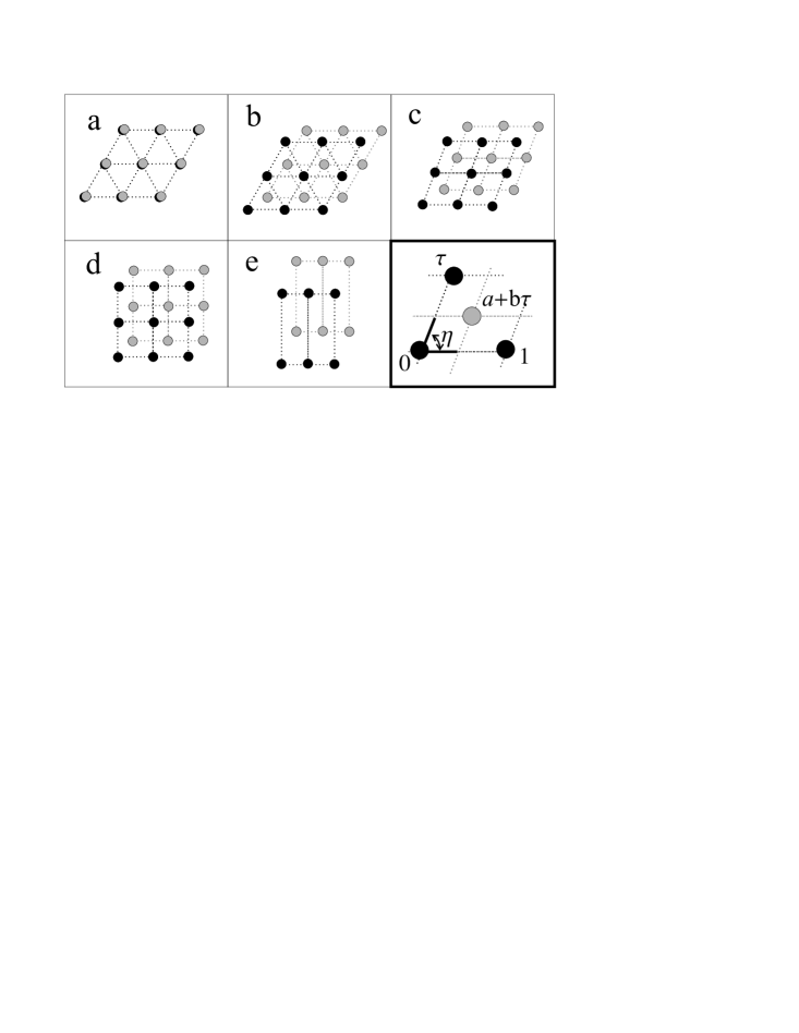
FIG. 1.: Phases of the two-component lattice: black and grey dots represent vortices of each of the two fluids. The panels a) through e) show the vortex structure in each of the phases described in the text. The final panel depicts the geometry of the lattices; the black and grey dots respectively occupy positions in the complex plane $\{m+n\tau\}$, and $\{(a+m)+(b+n)\tau\}$, where $m,n$ are integers. All minimal-energy configurations have $a=b$.

Refer to caption


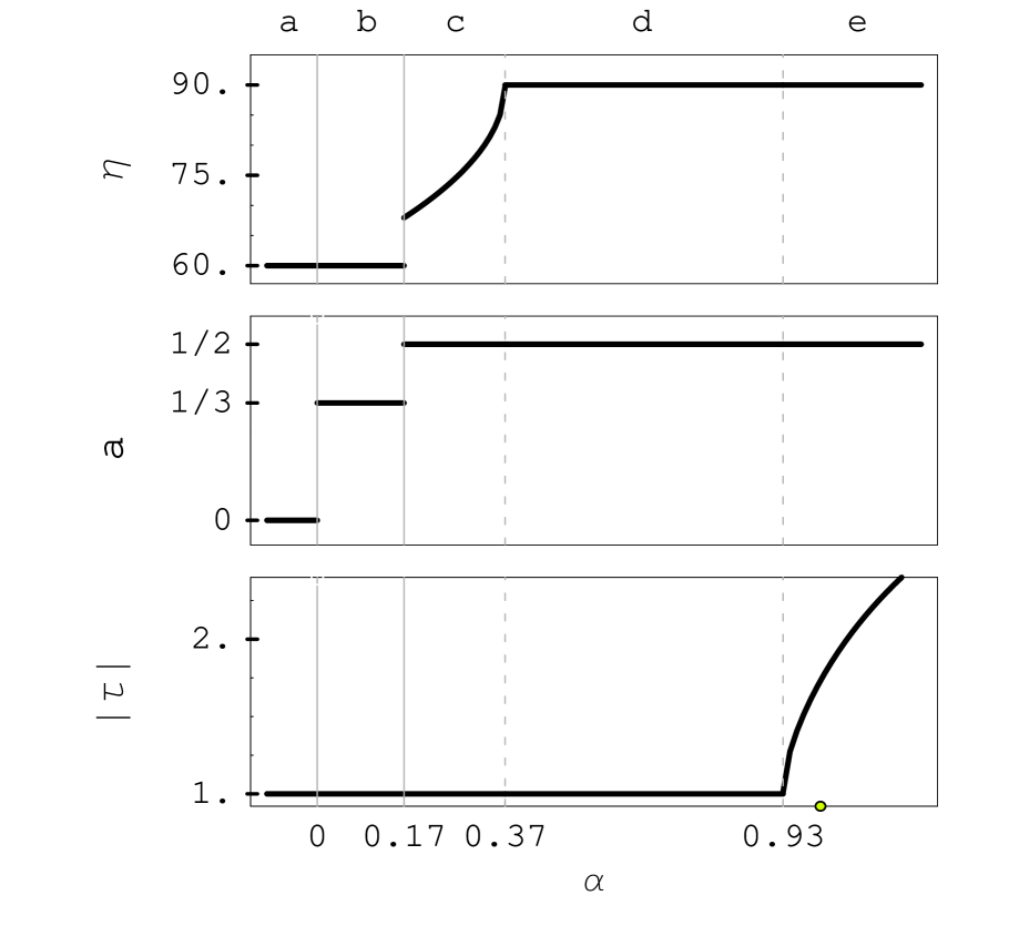
FIG. 2.: The parameters of the vortex lattice as a function of $\alpha=g_{12}/\sqrt{g_{1}g_{2}}$, a measure of the importance of interactions between unlike atoms. The phases, labeled a through e are illustrated in Fig. 1 along with the parameters $\tau=|\tau|e^{i\eta}$ and $a$. Solid and dashed vertical lines respectively denote first and second order phase transitions. The open circle on the horizontal axis indicates $\alpha=1$.