The effects of magnetic field on the $d$-density wave order in the cuprates

Abstract

We consider the effects of a perpendicular magnetic field on the $d$-density wave order and conclude that if the pseudogap phase in the cuprates is due to this order, then it is highly insensitive to the magnetic field in the underdoped regime, while its sensitivity increases as the gap vanishes in the overdoped regime. This appears to be consistent with the available experiments and can be tested further in neutron scattering experiments. We also investigate the nature of the de Haas- van Alphen effect in the ordered state and discuss the possibility of observing it.

Recently it was arguedChakravarty1 ; Chakravarty2 that the observed pseudogap in the cuprate superconductors is due to the development of a second type of order, the $d$-density wave order (DDW), which is a particle-hole condensate with an internal “angular momentum” 2. The notion of this broken symmetry has allowed us to understand an array of experiments, although a priori there is no sense in which such a state is close to, or adiabatically continuable to, a superconductor, or a Fermi liquid, which are the two most prominent states of matter.

From considerations of the simplest Hartree-Fock Hamiltonian that captures the broken symmetry of the DDW and the electromagnetic gauge invariance, we study the dependence of the DDW order parameter as a function of the applied magnetic field perpendicular to CuO-planes. We find that the effect of the magnetic field on the pseudogap is rather weak, if the DDW order is well-developed. For example, to destroy a DDW gap of magnitude of order 20 meV would require fields of order 1000 T, or larger. Moreover, this gap is highly insensitive to fields of order 25 T. This is, of course, a characteristic of the underdoped regime. In the overdoped regime, where the DDW gap drops rapidly to zero, the dependence on the magnetic field could be substantial.

We suggest that the recent neutron scattering experiments, which report a tantalizing evidence of DDW orderMook in the form of a resolution-limited elastic Bragg peak at the in-plane wave vector $(\pi/a,\pi/a)$, where $a$ is the lattice spacing, should be carefully examined for its dependence on a perpendicular magnetic field. The prediction is that the Bragg scattering intensity will be hardly affected, if the zero temperature DDW gap is substantial.Mook2

The effect of magnetic field on a superconductor is well known. Since the Cooper pairs involve time reversed mates, the effect of any time reversal breaking perturbation is very important. In contrast, the particle-hole pairs of the same spin orientation form the DDW condensate, and, as a consequence, such a condensate is inherently less affected by a magnetic field.

The contrasting response of a $d$-wave superconductor (DSC) and a DDW to applied magnetic field is further illuminated by examining the nodal quasiparticles of these two systems. The nodal quasiparticles of a DSC do not form Landau levels,Tesanovic while those of a DDW state do.Nersesyan This implies that, in principle, it is possible to observe de Haas-van Alphen (dHvA) oscillations in a DDW state, but not in a $d$-wave superconductor. The reason is that quasiparticles in a superconductor do not couple simply to the vector potential $\bf A$ corresponding to the magnetic field ${\mathbf{B}}={\bm{\nabla}}\times{\mathbf{A}}$, but to the supercurrent $(\bm{\nabla}\varphi-2e{\mathbf{A}}/\hbar c)$, where $\varphi$ is the phase of the superconducting order parameter, $e$ is the electronic charge, and $c$ is the velocity of light. We calculate dHvA oscillations of the magnetization in the DDW state and find that although $\Delta B/B$ could be of reasonable magnitude, the amplitude of the magnetization oscillations is weak, generically of order 0.01$\mu_{B}$. Thus, observation of these oscillations may be difficult.

Consider the mean field Hamiltonian of a $d$-density wave subjected to a magnetic field applied perpendicular to the plane. With the choice of the Landau gauge, the Peierls substituted Hamiltonian is written as:

$$H= - \mu\sum_{m,n}c^{+}_{m,n}c_{mn}-t\sum_{m,n}\left(c^{+}_{m,n}c_{m+1,n}+\text{h.c}\right)$$

$$- t\sum_{m,n}\left(e^{2\pi i\alpha m}c^{+}_{m,n}c_{m,n+1}+\text{h. c.}\right)$$

$$- \sum_{m,n}(-1)^{m+n}\Delta\left(-ic^{+}_{m,n}c_{m+1,n}+\text{h.c}\right)$$

$$+ \sum_{m,n}(-1)^{m+n}\Delta\left(-ie^{2\pi i\alpha m}c^{+}_{m,n}c_{m,n+1}+\text{h. c.}\right)$$

Here $m$ and $n$ are the site labels of a square lattice in the $x$- and $y$-directions; $\alpha=\phi/\phi_{0}$ is the magnetic flux through each plaquette of the square lattice in terms of the flux quantum $\phi_{0}=hc/e$, and $c_{m,n}$ is the fermion destruction operator at the site $(m,n)$. Here on, the hopping matrix element $t$ will be set to unity. The DDW gap satisfies the self-consistency condition:

$$\Delta=-i(-1)^{m+n}V\langle c^{+}_{m,n}c_{m+1,n}-\text{h. c.}\rangle,$$ (2)

where the angular brackets denote the groundstate average. Due to the conservation of current, ensured by the gauge invariance of the Hamiltonian (LABEL:eq:Hamiltonian), the DDW gap could as well be:

$$\Delta=i(-1)^{m+n}V\langle e^{2\pi i\alpha m}c^{+}_{m,n}c_{m,n+1}-\text{h. c.}\rangle.$$ (3)

Since a uniform applied magnetic field cannot break translational invariance, all physical quantities must be translationally invariant. Here $V$ is an energy parameter that controls the strength of DDW pairing.

We rewrite the Hamiltonian in terms of the Fourier transformed variables, given by (with lattice constant set to unity)

$$c_{m,n}=\frac{1}{\sqrt{N}}\sum_{k_{x},k_{y}}c_{k_{x},k_{y}}e^{i(k_{x}m+k_{y}n)},$$ (4)

where $N$ is the total number of sites on the lattice, to get

$$H = -\mu\sum_{k_{x},k_{y}}c^{\dagger}_{k_{x},k_{y}}c_{k_{x},k_{y}}-2\sum_{k_{x},k_{y}}\cos k_{x}c^{\dagger}_{k_{x},k_{y}}c_{k_{x},k_{y}}$$ (5)

$$- \sum_{k_{x},k_{y}}\left(e^{ik_{y}}c^{\dagger}_{k_{x}+2\pi\alpha,k_{y}}c_{k_{x},k_{y}}+\text{h. c.}\right)$$

$$+ \Delta\sum_{k_{x},k_{y}}\left(ie^{ik_{x}}c^{\dagger}_{k_{x}+\pi,k_{y}+\pi}c_{k_{x},k_{y}}+\text{h. c.}\right)$$

$$- \Delta\sum_{k_{x},k_{y}}\left(ie^{ik_{y}}c^{\dagger}_{k_{x}+\pi+2\pi\alpha,k_{y}+\pi}c_{k_{x},k_{y}}+\text{h. c.}\right).$$

One sees immediately that the states $(k_{x},k_{y})$, $(k_{x}+2\pi\alpha,k_{y})$, $(k_{x}+4\pi\alpha,k_{y})$, …, $(k_{x}+\pi,k_{y}+\pi)$, $(k_{x}+\pi+2\pi\alpha,k_{y}+\pi)$, $(k_{x}+\pi+4\pi\alpha,k_{y}+\pi)$, … are coupled. For rational flux, $\alpha=p/q$, where $p$ and $q$ are relative primes, the set of coupled states is finite, containing $2q$ elements. At this point, the connection to the Hofstadter problemHofstadter becomes particularly obvious. The Hamiltonian can be written as the following quadratic form:

$$H=\sum_{\bf k}\Psi_{\bf k}^{\dagger}(H_{\bf k}-\mu)\Psi_{\bf k},$$ (6)

where $k_{x}\in[0,2\pi\alpha)$ and $k_{y}\in[0,\pi)$. The row vector $\Psi_{\bf k}^{T}$ is given by

$$\begin{split}\Psi_{\bf k}^{T}=(&c_{k_{x},k_{y}},c_{k_{x}+2\pi\alpha,k_{y}},c_{k_{x}+4\pi\alpha,k_{y}},\ldots,c_{k_{x}+2\pi\alpha(q-1),k_{y}},\\ &c_{k_{x}+\pi,k_{y}+\pi},c_{k_{x}+\pi+2\pi\alpha,k_{y}+\pi},c_{k_{x}+\pi+4\pi\alpha,k_{y}+\pi},\ldots,\\ &c_{k_{x}+\pi+2\pi\alpha(q-1),k_{y}+\pi}),\end{split}$$

and the matrix $H_{\bf k}$ is

$$\begin{vmatrix}-2\cos k_{x}&-e^{-ik_{y}}&0&\ldots&-e^{ik_{y}}&-2i\Delta\cos k_{x}&i\Delta e^{-ik_{y}}&0&\ldots&i\Delta e^{ik_{y}}\\ -e^{ik_{y}}&-2\cos(k_{x}+2\pi\alpha)&-e^{-ik_{y}}&\ldots&0&i\Delta e^{ik_{y}}&-2i\Delta\cos(k_{x}+2\pi\alpha)&i\Delta e^{-ik_{y}}&0&\ldots\\ 0&-e^{ik_{y}}&-2\cos(k_{x}+4\pi\alpha)&\ldots&&0&i\Delta e^{ik_{y}}&\ldots&\ldots&\dots\\ \vdots&&\ddots&&&\vdots&&\ddots&\\ 2i\Delta\cos k_{x}&-i\Delta e^{-ik_{y}}&0&\ldots&-i\Delta e^{ik_{y}}&2\cos k_{x}&e^{-ik_{y}}&0&\ldots&e^{ik_{y}}\\ -i\Delta e^{ik_{y}}&2i\Delta\cos(k_{x}+2\pi\alpha)&-i\Delta e^{-ik_{y}}&0&\ldots&e^{ik_{y}}&2\cos(k_{x}+2\pi\alpha)&e^{-ik_{y}}&\ldots&0\\ 0&-i\Delta e^{ik_{y}}&\ldots&\ldots&\dots&0&e^{ik_{y}}&&\ldots\\ \vdots&&&&&\vdots\end{vmatrix}$$ (7)

The gap satisfies the equation

$$\Delta = \frac{V}{N}\sum_{\bf k}\left[\langle-ie^{ik_{x}}c^{\dagger}_{k_{x}+\pi,k_{y}+\pi}c_{k_{x},k_{y}}\rangle+\text{h. c.}\right]$$ (8)

$$= \frac{V}{N}\sum_{\bf k}\Delta_{\bf k}.$$

For each value of $(k_{x},k_{y})$, the Hamiltonian was diagonalized, giving rise to a new set of fermion operators $\{d_{\bf k}^{i}\}$, $i=1,\ldots,2q$. Then, $\Delta_{k_{x},k_{y}}$, $\Delta_{k_{x}+2\pi\alpha,k_{y}}$, …, $\Delta_{k_{x}+2\pi\alpha(q-1),k_{y}}$, $\Delta_{k_{x}+\pi,k_{y}+\pi}$, $\Delta_{k_{x}+\pi+2\pi\alpha,k_{y}+\pi}$, …, $\Delta_{k_{x}+\pi+2\pi\alpha(q-1),k_{y}+\pi}$ were computed and so was the energy spectrum. Several values of $k_{x}$ and $k_{y}$ were chosen in the sub-Brillouin zone (sBZ) and finally the gap was obtained as

$$\Delta=\frac{1}{2qN_{x}N_{y}}\sum_{{\bf k}\in\text{sBZ}}\Delta_{\bf k},$$ (9)

where $N=(qN_{x})(2N_{y})$. The whole process was repeated until $\Delta$ converged.

Typical magnetic fields in laboratories are of order $20\,T$, equivalent to $(1/1225)\phi_{0}$ for the cuprates with lattice spacing of $4$ Å. In our computation, we were able to diagonalize matrices of size $4000\times 4000$, or $q=2000$ corresponding to the smallest field of $12.5\,T$. Since the gap is so insensitive to the applied field, going to smaller fields appeared unnecessary.

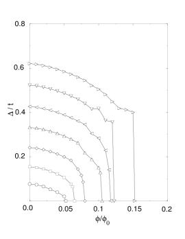
Figure 1: The DDW gap magnitude $\Delta$ as a function of the applied flux $\phi/\phi_{0}$ for various values of the coupling strength $V/t$ ($\bigcirc:0.5$; $\Box:0.75$; $\Diamond:1.0$; $\bigtriangleup:1.25$; $\triangleleft:1.5$; $\bigtriangledown:1.75$; $\triangleright:2.0$) for $\mu=-0.1t$.

In Fig. 1, we show the dependence of the DDW gap versus magnetic field at absolute zero for $\mu=-0.1t$ as a function of $V$. We observe a striking insensitivity of the gap with respect to the magnetic field. The gap only collapses, through a first-order transition at a flux strength $\phi_{c}/\phi_{0}$, corresponding to a large laboratory magnetic field ($\phi_{0}\approx 25,000$T for cuprates). The gaps at zero field was calculated separately, and the results for finite field were seen to converge to them as $\phi\to 0$. It is important to note that because the chemical potential is finite, the DDW transition does not take place at $V=0^{+}$, but at a finite threshold value $V_{c}$. This is clearly seen in Fig. 2.

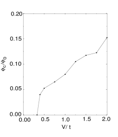
Figure 2: The critical field as a function of $V$ for $\mu=-0.1t$.

In the same figure, we see that $\phi_{c}/\phi_{0}$ drops quite rapidly to zero as $V_{c}$ is approached. Thus, although $\phi_{c}$ corresponds to quite large magnetic fields when the DDW gap is large in the underdoped regime, it could be quite small when the gap is small in the overdoped regime. For a gap of order 20 meV, the critical magnetic field is of order 1250 T.

In order to test the correctness of our computations, we also calculated the groundstate energy density at half-filling ($\mu=0$). We observe an increase in the groundstate energy as the magnetic field is applied; this increase indicates a diamagnetism in the DDW system. This result has, in fact, been analytically derived Nersesyan using the nodal fermi gas formalism of the DDW state for $\mu=0$. In particular, it was shown that the DDW groundstate energy, expressed in terms of lattice parameters, behaves as

$$E_{GS}(\phi)=E_{GS}(0)+2\frac{\zeta(3/2)}{\sqrt{\pi}}\,A\,t\,\sqrt{\frac{W}{t}}\left(\frac{\phi}{\phi_{0}}\right)^{3/2},$$ (10)

where $\zeta(x)$ is Riemann’s zeta function, $A$ and $W$ being the system area and a cutoff energy. The above formula is expected to hold only for small fields such that $\hbar\omega_{c}=\hbar eB/m^{*}c<<W$. This appears to be a surprisingly robust result, as shown in Fig. 3, especially because we made no approximations involving nodal Fermions. The fit at the smallest field gave a sensible $W=1.6t$. The quantity $W$ was interpreted in Ref. Nersesyan, as the cutoff energy below which the Dirac fermion description holds for the DDW state.

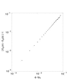
Figure 3: The groundstate energy as a function of the applied magnetic field at $\mu=0$.

As a consequence of the nonanalytic field dependence of the energy at $\mu=0$, the diamagnetic susceptibility diverges at zero field: $\chi\propto B^{-1/2}$. Obviously, this divergence poses a serious question about the stability of the DDW state at $\mu=0$. It is clear, however, that this divergence will be cut off for a finite chemical potential, $\mu\neq 0$. Similarly, the divergence will also be removed at finite temperatures even for $\mu=0$. Moreover, three dimensional coupling between the layers will also modify the result for the susceptibility.Nersesyan It is important to stress that the divergence in the susceptibility is intimately related to the appearance of zero-energy modes, which is a direct consequence of the nodal points and the doubling of the Dirac fermions.

It has recently been proposed in Ref. Balatsky, that a finite magnetic field may induce an additional $d_{xy}$ gap. Such a gap can efficiently remove the nodes and hence the divergence in the diamagnetic susceptibility. However, the small $d_{xy}$ gap will not be manifest at a finite temperature and the dominant cutoff will be provided by the temperature or the chemical potential. Therefore our computation for the DDW gap retains its relevance to experimental situations.

As an interesting contrast to DSC, an essential feature of the Dirac fermion picture of the DDW is the formation of Landau levels in a magnetic field:Nersesyan $E_{n}=\sqrt{n(\hbar\omega_{c})\Delta_{0}}$, where $\Delta_{0}$ is the amplitude of the gap, and $\omega_{c}$ is the cyclotron frequency, $eB/m^{*}c$, $m^{*}$ being the effective mass corresponding to the nodal region. As a result, the DDW system away from half-filling is expected to exhibit de Haas-van Alfven (dHvA) oscillations in the magnetization.

For a free electron system at chemical potential $\mu$, where the energy spacing is $\hbar\omega_{c}$, the oscillation frequency satisfies

$$\frac{\Delta B}{B}=-B\Delta\left(\frac{1}{B}\right)=\frac{\hbar\omega_{c}}{|\mu|}.$$ (11)

Taking $B=1\,T$, $\mu\approx 0.25\,eV$, one would get $\Delta B\approx 5\,G$. For nodal fermi gas at chemical potential $\mu$, the oscillation frequency is

$$\frac{\Delta B}{B}=-B\Delta\left(\frac{1}{B}\right)=(\frac{\hbar\omega_{c}}{|\mu|})(\frac{\Delta_{0}}{|\mu|}).$$ (12)

To make an estimate, we can choose $B=1\,T$. It is more problematic to estimate $\mu$ in the underdoped regime in which the DDW state is likely to be found, and in which the typical non-interacting band picture may not hold. There is some evidence, however, that $\mu\approx-tx^{2}$, where $x$ is the doping.Sumanta Choosing $x\approx 0.15$, $\Delta_{0}$ of the order of the pseudogap $\sim 20$ meV, and $t\approx 0.25$ eV, results in $\Delta B\approx 0.05$ T, which is clearly within the detectable range of dHvA oscillation experiments.

The above estimate for $\Delta B$ is not sufficient for the detectability of dHvA effect. We must also estimate the magnitude of the magnetization oscillations. For this purpose, it is convenient to consider energy spectrum of the nodal fermions of the DDW state.

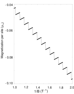
Figure 4: The de Haas-van Alphen oscillations of the magnetization in the DDW state.

The oscillation in energy, and thus of the magnetization, occurs whenever a Landau level passes through the Fermi level. For hole-doped cuprates, with a finite chemical potential $\mu$, the formula (10) for the groundstate energy must be augmented by the following additional term:

$$\frac{eB}{hc}\sqrt{\hbar\omega_{c}\Delta_{0}}\ \sum_{n=0}^{n_{\mu}}\sqrt{n}$$ (13)

where $[n_{\mu}]$ is the largest integer smaller than $\mu^{2}/(\hbar\omega_{c}\Delta_{0})$. In other words, $n_{\mu}$ is the number of filled Landau levels. With the above choice of parameters, the magnetization per unit cell, in units of Bohr magneton, $\mu_{B}$, is shown in Fig. 4. In plotting this figure, we have removed the spurious $\delta$-function singularities arising from taking derivatives of the step functions. At finite temperature, the sharpness of the oscillations will be smoothed out, but the oscillation amplitude will still roughly be of order $\approx 0.01\,\mu_{B}$, which is quite weak. As is evident from Fig. 4, as the magnetic field swept between $0.5$ T and $1$ T, the system undergoes about $14$ oscillations.

There are already some experiments that appear to shed light on the effect of magnetic field on the pseudogap. Nuclear magnetic resonance experiments in underdoped $\mathrm{YBa_{2}Cu_{4}O_{8}}$ clearly support the view that the pseudogap is hardly affected by an applied perpendicular magnetic field,Zheng and so does experimets in nearly optimally dopedPennington $\mathrm{YBa_{2}Cu_{3}O_{7-\delta}}$. In contrast, nuclear magnetic resonance experiments in overdoped $\mathrm{TlSr_{2}CaCu_{2}O_{6.8}}$ provides contrasting evidence that in this regime the pseudogap is sensitive to the magnetic field.Zheng2 At first sight, the experiments in $\mathrm{YBa_{2}Cu_{3}O_{7-\delta}}$ appear to be controversial because there are also reports to the contrary,NMR2 ; NMR3 but as was pointed out by the authors of Ref. Zheng2, , the later reports by the authors of Ref. NMR2, ; NMR3, seem to be in agreement with Ref. Pennington, . Therefore, our theoretical results would be consistent with experiments, if the pseudogap is indeed caused by DDW. We hope that our work will catalyse further experiments on this important question. On the theoretical front, it will be necessary to go beyond the Hartree-Fock approximation, especially at finite temperatures. To go beyond Hartree-Fock approximations, we must recognize the fact that the DDW gap, which characterizes the orbital currents need not be in the perfect staggered pattern, but can be flipped as long as the current conservations at the vertices are satisfied.Chakravarty We hope to report on this issue in the future.

We thank A. V. Balatsky, Pengcheng Dai, H. A. Mook, and C. Nayak for interesting discussions. This work was supported by a grant from the National Science Foundation: NSF-DMR-9971138.

References

- (1) S. Chakravarty and H. Y. Kee, Phys. Rev. B 61, 14821 (2000).
- (2) S. Chakravarty, R. B. Laughlin, D. K. Morr, and C. Nayak, Phys. Rev. B 64, 094503 (2001).
- (3) H. A. Mook, P. Dai, and F. Dogan, Phys. Rev. B 64, 012502 (2001), and H. A. Mook et al., in preparation. For a theoretical analysis of these experiments, see S. Chakravarty, H. -Y. Kee, and C. Nayak, Int. J. Mod. Phys. 15, 2901 (2001)and cond-mat/0112109.
- (4) Preliminary results indicate that this is indeed may be the case (H. A. Mook, private communications).
- (5) M. Franz and Z. Tesanović, Phys. Rev. Lett. 84, 554 (2000).
- (6) A. A. Nersesyan and G. E. Vachnadze, J. of Low Temp. Phys. 77, 293 (1989); see also, X. Yang and C. Nayak, cond-mat/0108407.
- (7) D. R. Hofstadter, Phys. Rev. B 14, 2239 (1976).
- (8) J-H. Zhu and A. V. Balatsky, cond-mat/0110214.
- (9) The choice of this chemical potential was discussed in S. Tewari, H. -Y. Kee, C. Nayak, and S. Chakravarty, Phys. Rev. B 64, 224516 (2001).
- (10) Guo-quing Zheng, W. G. Clark, Y. Kitaoka, K. Asayama, Y. Kodama, P. Kuhns, and W. G. Moulton, Phys. Rev. B 60, R9947 (1999).
- (11) K. Gorny, O. M. Vyaselev, J. A. Martindale, V. A. Nandor, C. H. Pennington, P. C. Hammel, W. L. Hults, J. L. Smith, P. L. Kuhns, A. P. Reyes, and W. G. Moulton, Phys. Rev. Lett. 82, 177 (1999).
- (12) Guo-quing Zheng, H. Ozaki, W. G. Clark, Y. Kitaoka, P. Kuhns, A. P. Reyes, W. G. Moulton, T. Kondo, Y. Shimakawa, and Y. Kubo, Phys. Rev. Lett. 85, 405 (2000).
- (13) V. F. Mitrović et al., Phys. Rev. Lett. 82, 2784 (1999); H. N. Bachman et al., Phys. Rev. B 60, 7591 (1999).
- (14) P. Carretta et al., Phys. Rev. B 61, 12420 (2000); 54, R99682 (1996).
- (15) The finite temperature behavior is that of the six-vertex model (S. Chakravarty, unpublished).