[

Quantum computing of molecular magnet Mn₁₂

Abstract

Quantum computation in molecular magnets is studied by solving the time-dependent Schrödinger equation numerically. Following Leuenberger and Loss (Nature (London) 410, 789(2001)), an external oscillating magnetic field is applied to populate and manipulate the spin coherent states in molecular magnet Mn₁₂. The conditions to realize parallel recording and reading data bases of Grover algorithsm in molecular magnets are discussed in details. It is found that an accurate duration time of magnetic pulse as well as the amplitudes are required to design the device of quantum computing.

]

Quantum phase was proposed to store information in connection with a new class of computational algorithms based on the rules of quantum mechanics rather than classical physics.[1] One example is the database search problem proposed by Grover.[2, 3] Differing from other quantum algorithms, the superposition of single-particle quantum states is sufficient for Grover’s algorithm. The Grover’s algorithm was successfully implemented using Rydberg atoms.[4] Recently, Leuenberger and Loss theoretically proposed that molecular magnets Mn₁₂ can be used to realize the Grover’s algorithm by utilizing multifrequency coherent magnetic radiation.[5] In the S-matrix and time-dependent high-order perturbation theory, they showed that it was possible to populate and manipulate spin coherent excited states by applying a single pulse of weak oscillating transverse magnetic field with an appropriate number of matching frequencies, and  the coherent state can be applied for storing a multi-bites information. In this paper the population and manipulation of a spin coherent excited state in an external oscillating magnetic field is studied by solving the time-dependent Schrödinger equations numerically. The conditions for the field to implement the Grover’s algorithm are discussed in details. We find that an accurate duration time of magnetic pulse as well as the oscillating frequencies and amplitudes are required to design the device of quantum computing in the molecular magnets Mn${}_{12}.$

Following Leuenberger and Loss, we consider a molecular magnet with spin $S$ $(>1/2)$ in presence of a weak oscillating transverse magnetic field. The Hamiltonian for the system reads

$$H=H_{\text{spin}}+V_{\text{low}}(t)+V_{\text{high}}(t),$$ (1)

where

$$H_{\text{spin}}=-AS_{z}^{2}-BS_{z}^{4}+g\mu_{B}\delta H_{z}S_{z},$$ (2)

$$V_{\text{low}}(t)=g\mu_{B}H_{0}(t)\cos(\omega_{0}t)S_{z},$$ (3)

$$V_{\text{high}}(t) = \sum_{m=m_{0}}^{s-1}\frac{g\mu_{B}H_{m}(t)}{2}$$ (5)

$$\times\left[e^{i(\omega_{m}t+\Phi_{m})}S_{+}+e^{-i(\omega_{m}t+\Phi_{m})}S_{-}\right].$$

$H_{\text{spin}}$ is a single spin Hamiltonian for molecular magnet Mn${}_{12}.$[6] $\left|m\right\rangle$ are the simultaneous eigenstates of $H_{\text{spin}}$ and the z-component spin operator ${\bf S}_{z}$ with the energy $\varepsilon_{m}$ and the moment $m\hbar$. $V_{\text{low}}$ and $V_{\text{high}}$ are the Zeeman terms to describe the coupling between the external magnetic fields and the spin S. The low frequency is applied along the easy axis, and $V_{\text{low}}$ supplies the necessary energy for the resonance condition. The high frequency transverse fields are introduced to induce the transition from the initial state $\left|s\right\rangle$ to virtual states $\left|m\right\rangle,$ $m=m_{0},\cdots,s-1,$ and the frequencies $\omega_{m}$, $m=m_{0},\cdots,s-2,$ mismatch the level separation by $\omega_{0}$, that is , $\hbar\omega_{m}=\varepsilon_{m}-\varepsilon_{m+1}+\hbar\omega_{0},$ and $\omega_{s-1}=$ $\varepsilon_{s}-\varepsilon_{s+1}+(s-m_{0}-1)\hbar\omega_{0}.$ The phases $\Phi_{m}=\sum_{k=s-1}^{m+1}\Phi_{k}+\varphi_{m\text{ }}$($\varphi_{m\text{ }}$ is the relative phase) and

$\displaystyle H_{m}(t)=\left\{\begin{array}[]{l}H_{m},\text{ if }t\in(-\frac{T}{2},\frac{T}{2})\text{ for }m=0\text{ and }m\geq m_{0},\\ 0,\text{ otherwise.}\end{array}\right.$

The time-dependent Schrödinger equation reads

$$i\hbar\frac{\partial}{\partial t}\left|\Psi(t)\right\rangle=H\left|\Psi(t)\right\rangle,$$ (6)

where

$$\left|\Psi(t)\right\rangle=\sum_{m=m_{0}}^{s}a_{m}(t)e^{-i\varepsilon_{m}t/\hbar}\left|m\right\rangle$$ (7)

The eigenstates of $m<m_{0}$ have been neglected. The molecular magnets Mn₁₂ behaves like single spin, and has a ground state with spin $s=10$.

The Grover scheme becomes adapted to describe the quantum computational read-in and decoding of the quantum data register ${\bf a=(}a_{s},a_{s-1},...,a_{m_{0}}).$ Firstly, as a simplest example, let us discuss the case of $m_{0}=9.$ At the first stage of the so called “read-in”, the initial values of $\{a_{m}^{(0)}:m=10,9\}$ are set to be $\{a_{10}^{\left(0\right)}=1$, $a_{9}^{\left(0\right)}=0\}.$ After irradiating the molecular magnets Mn₁₂ with a coherent magnetic pulse with the relative phase $\varphi_{9}^{(1)}$ in the duration time $T$, one has the quantum data register ${\bf a=(}a_{10}^{(1)},a_{9}^{(1)})$ with

$$a_{10}^{(1)}=\cos\left(\frac{g\mu_{B}H_{9}}{2\hbar}\langle 9|S_{-}|10\rangle T\right),$$ (8)

$$a_{9}^{\left(1\right)}=-ie^{-i\varphi_{9}^{(1)}}\sin\left(\frac{g\mu_{B}H_{9}}{2\hbar}\langle 9|S_{-}|10\rangle T\right).$$ (9)

At the second stage of the so called “decoding”, the solutions of (8) and (9) become the initial values of $\{a_{m}\}$ in Eq.(6), and the relative phase is set to be $\varphi_{9}^{(2)}=0.$ At the end of decoding, one obtains

$$a_{9}^{(2)}=\left\{\begin{array}[]{l}-i\sin\left(2\frac{g\mu_{B}H_{9}}{2\hbar}\langle 9|S_{-}|10\rangle T\right),\text{ \quad for }\varphi_{9}^{(1)}=0\\ 0,\text{ \qquad\qquad\qquad\qquad\qquad\qquad for }\varphi_{9}^{(1)}=\pi\end{array}\right.$$ (10)

If the condition of $g\mu_{B}H_{9}\langle 9|S_{-}|10\rangle T/2\hbar\ll 1$ is satisfied, the result in Eq. (10) is in a good consistence with Ref.[5]. For a longer duration time $T\gg\left[g\mu_{B}H_{9}\langle 9|S_{-}|10\rangle/2\hbar\right]^{-1},$the condition fails to implement the Grover algorithm.

For $m_{0}<9$, it is difficult to solve Eq.(6) analytically. However, as it is a single particle problem only relating to a finite number of states, it is possible for us to solve the differential equations numerically instead of evaluating the S-matrix perturbatively as Leuenberger and Loss did. The results of explicit numerical calculation should be more reliable than other approximate results. For illustration, we focus on the case $m_{0}=5.$ The parameters used here are the same as the ones in Ref.[5]: $\omega_{0}=5\times 10^{7}s^{-1}$, $T=10^{-7}s$, $H_{0}=H_{9}=2G$, $H_{8}/H_{0}=-0.04,$ $H_{7}/H_{0}=-0.25,$ $H_{6}/H_{0}=-0.61,$ and $H_{5}/H_{0}=-1.12$. For the molecular magnets Mn₁₂, $A$ and $B$ in Eq.(2) are $0.56K$ and $1.11\times 10^{-3}K,$ respectively.[6] According to the Ref.[5], the relative phases are $\varphi_{9}^{(1)}=\varphi_{8}^{(1)}=\varphi_{7}^{(1)}=0$ and $\varphi_{6}^{(1)}=\varphi_{5}^{(1)}=\pi$ for encoding the number $13_{10}=1101_{2}.$ Now, we solve six first-order differential equations for $\{a_{m}(t)\}$ in Eq. (7). The initial values of the $\{a_{m}\}$ are set to be $a_{10}^{(0)}=1$ and $a_{m}^{(0)}=0$ for $m\neq 10$. After a duration time T, we have ${\bf a}^{(1)}{\bf=(}a_{10}^{(1)},a_{9}^{(1)},a_{8}^{(1)},a_{7}^{(1)},a_{6}^{(1)},a_{5}^{(1)}).$ At the second stage for decoding the number, ${\bf a}^{(1)}$ becomes the initial values of Eq.(6) and the relative phases should be set by $\varphi_{9}^{(2)}=\varphi_{7}^{(2)}=\varphi_{5}^{(2)}=0$ and $\varphi_{8}^{(2)}=\varphi_{6}^{(2)}=\pi$ . Once again, the six first-order differential equations with the new initial conditions are solved numerically. At the end of decoding, we obtain ${\bf a}^{(2)}{\bf=(}a_{10}^{(2)},a_{9}^{(2)},a_{8}^{(2)},a_{7}^{(2)},a_{6}^{(2)},a_{5}^{(2)}).$ If Grover’s algorithm is implemented successfully, according to Leuenberger and Loss, one should have $\left|a_{10}^{(2)}\right|\approx 1,\left|a_{9}^{(2)}\right|\approx 2\left|a_{9}^{(1)}\right|\approx 2\eta,$ $\left|a_{8}^{(2)}\right|\approx 0,$ $\left|a_{7}^{(2)}\right|\approx 2\left|a_{7}^{(1)}\right|\approx 2\eta,$ $\left|a_{6}^{(2)}\right|\approx 2\left|a_{6}^{(1)}\right|\approx 2\eta,$ $\left|a_{5}^{(2)}\right|\approx 0$ and $\eta\ll 1.$ Instead, our numerical calculation gives

$$\left|a_{10}^{(1)}\right| \approx 0.95,\text{ }\left|a_{9}^{(1)}\right|\approx 0.31,\text{ }\left|a_{8}^{(1)}\right|\approx 0.04,\text{ }$$

$$\left|a_{7}^{(1)}\right| \approx 0.01,\text{ }\left|a_{6}^{(1)}\right|\approx 0.02,\text{ }\left|a_{5}^{(1)}\right|\approx 0.01$$

and

$$\left|a_{10}^{(2)}\right| \approx 0.82,\text{ }\left|a_{9}^{(2)}\right|\approx 0.59,\text{ }\left|a_{8}^{(2)}\right|\approx 0.08,$$

$$\left|a_{7}^{(2)}\right| \approx 0.06,\text{ }\left|a_{6}^{(2)}\right|\approx 0.01,\text{ }\left|a_{5}^{(2)}\right|\approx 0.01.$$

The values of $\{a_{m}^{(1)},a_{m}^{(2)}\}$ are complex numbers (not real) and we only present their absolute values here. Therefore, the numerical solution shows that the encoding number likes $0001_{2},$ but is not $1101_{2}$ as expected by Leuenberger and Loss at the specific values of applied field and duration time $T$ . However, $\{a_{m}^{(1)},a_{m}^{(2)}\}$ depend on the duration time $T$, and one may be still able to reach to the encoding number $1101_{2}$ by a specific duration time $T$ of pulse.

To clarify the feasibility of the method proposed by Leuenberger and Loss, we study a simple, but nontrivial case of $m_{0}=8$ as a representative example. The key approximations in Leuenberger and Loss’s method are that $S_{m,s}^{(j)}=0$ for $j<n(=s-m_{0})$. The transitions from $|k\rangle$ to $|m\rangle$, i.e. $S_{m,k}^{(j)}$ $(m<k<s)$ and all higher order amplitudes $S_{m,s}^{(j)}$ are neglected. In the case of $m_{0}=8$, the first order perturbation are required to be zero: $S_{9,10}^{(1)}=S_{8,9}^{(1)}=0,$ or at least $\left|S_{9,10}^{(1)}\right|\ll\left|S_{9,10}^{(2)}\right|(\simeq\left|S_{8,10}^{(2)}\right|)$ and $\left|S_{8,9}^{(1)}\right|\ll\left|S_{9,10}^{(2)}\right|(\simeq\left|S_{8,10}^{(2)}\right|).$ In fact, the quantum amplitudes of the transitions by the perturbative $S-$matrix formula are given by

$$S_{9,10}^{(2)}=\frac{2\pi}{i}\left(\frac{g\mu_{B}}{2\hbar}\right)^{2}\frac{H_{0}H_{9}e^{i\Phi_{9}}}{\omega_{0}}\langle 9|S_{-}|10\rangle\frac{T}{2\pi}$$ (11)

$$S_{8,10}^{(2)}=\frac{2\pi}{i}\left(\frac{g\mu_{B}}{2\hbar}\right)^{2}\frac{H_{8}H_{9}e^{i\Phi_{8}}e^{i\Phi_{9}}}{\omega_{0}}\langle 8|S_{-}|9\rangle\langle 9|S_{-}|10\rangle\frac{T}{2\pi}$$ (12)

$$S_{9,10}^{(1)}=\frac{1}{i}\frac{g\mu_{B}H_{9}e^{i\Phi_{9}}}{2\hbar}\langle 9|S_{-}|10\rangle\frac{\sin(\omega_{0}T/2)}{\omega_{0}/2}$$ (13)

$$S_{8,9}^{(1)}=\frac{1}{i}\frac{g\mu_{B}H_{8}e^{i\Phi_{8}}}{2\hbar}\langle 8|S_{-}|9\rangle\frac{\sin(\omega_{0}T/2)}{\omega_{0}/2}$$ (14)

where $\Phi_{9}=\varphi_{9}$ and $\Phi_{8}=\Phi_{9}+\varphi_{8}$ ($\varphi_{9}$ and $\varphi_{8}$ are the relative phase). The first two terms $\{S_{9,10}^{(2)},S_{8,10}^{(2)}\}$ result from the second perturbation contributions with energy conservation. From the condition $\left|S_{9,10}^{(2)}\right|\simeq\left|S_{8,10}^{(2)}\right|,$ one can deduce the field amplitude $H_{8}/H_{0}=0.16.$ However, the lower order terms $S_{9,10}^{(1)}$ and $S_{8,9}^{(1)}$ , in general, are not exactly equal to zero even if they do not satisfy the energy conservation. They can be zero only if $\omega_{0}T=2\pi l$ where $l$ is an integer. Due to these terms $S_{9,10}^{(1)}$ and $S_{8,9}^{(1)}$ , the amplitudes of the $a_{8}(t)$ and $a_{9}(t)$ in the state $\left|\Psi(t)\right\rangle$ are obviously oscillating with varying $T$. We have shown them in Fig. (1).

Now, let us assume the parameters: $T=1.0\times 10^{-9}$s, $H_{0}=200G$, $H_{9}=20G$ and $\omega_{0}=4\pi\times 10^{9}$s^-1. It gives $\left|S_{8,10}^{(2)}\right|\simeq 0.11.$ Following Leuenberger and Loss, we set $\varphi_{9}^{(2)}=0$ and $\varphi_{8}^{(2)}=0$. Then, the recording number $00_{2}$ corresponds to $\{\varphi$ ${}_{9}^{(1)}=\pi$, $\varphi_{8}^{(1)}=\pi\},$ $01_{2}$ to $\{\varphi_{9}^{(1)}=0$, $\varphi_{8}^{(1)}=\pi\},$ $10_{2}$ to $\{\varphi_{9}^{(1)}=\pi$, $\varphi_{8}^{(1)}=0\},$ and $11_{2}$ to $\{\varphi_{9}^{(1)}=0$, $\varphi_{8}^{(1)}=0\}.$ The results by our numerical calculation are shown in the Table 1 (where $m=9,8$ represent the binary digits $2^{0}$ and $2^{1},$ respectively).

Table 1: The numerical results for the case of $m_{0}=8$.

decoded number $\left|a_{10}^{(1)}\right|$ $\left|a_{9}^{(1)}\right|$ $\left|a_{8}^{(1)}\right|$ $\left|a_{10}^{(2)}\right|$ $\left|a_{9}^{(2)}\right|$ $\left|a_{8}^{(2)}\right|$ $00_{2}$ $0.99$ $0.13$ $0.10$ $1.00$ $0.07$ $0.01$ $01_{2}$ $0.99$ $0.13$ $0.10$ $0.96$ $0.26$ $0.04$ $10_{2}$ $0.98$ $0.14$ $0.10$ $0.98$ $0.04$ $0.20$ $11_{2}$ $0.98$ $0.14$ $0.10$ $0.94$ $0.28$ $0.19$

Using the above parameters, the proposal by Leuenberger and Loss can be implemented. However, the values $\{|a_{10}^{(2)}|,$ $|a_{9}^{(2)}|,$ $|a_{8}^{(2)}|\}$ are not constants and will be changed with the duration time $T$ of pulse. In a certain range, $\left|S_{9,10}^{(1)}\right|$ or $\left|S_{8,9}^{(1)}\right|$ will have the close magnitude to $\left|S_{m,s}^{(n)}\right|$, which can result in the deformation of the recording, or even in the destruction. In Fig.1 we plot amplitudes of $\left|a_{9}^{(2)}\right|$ and $\left|a_{8}^{(2)}\right|$ with varying $T$ (for $\varphi_{9}^{(1)}=0$ and $\varphi_{8}^{(1)}=\pi$) which corresponds to $01_{2}.$ The amplitudes $\left|a_{9}^{(2)}\right|\sim 0.26$ and $\left|a_{8}^{(2)}\right|\sim 0.04$ for a duration time $T=10^{-9}s.$ The value $0.26$ can be considered as a digit number $1$ and $\ 0.04$ as $0.$ The values $\left|a_{9}^{(2)}\right|$ and $\left|a_{8}^{(2)}\right|$ are varied with the pulse duration $T.$ The first maximum of $\left|a_{8}^{(2)}\right|$ $\sim 0.107$ at $T\sim 1.16$ $\times 10^{-9}s,$ the second maximum $\left|a_{8}^{(2)}\right|\sim 0.22$ at $T\sim 1.66$ $\times 10^{-9}s$ which becomes larger than the first minium of $\left|a_{9}^{(2)}\right|\sim 0.19$ at $T\sim 1.37$ $\times 10^{-9}s.$ Therefore, we conclude that a rather definite duration of pulse should be chosen for a stable and clear quantum recording.

One can straightforwardly extend the above discussion to the case of $m_{0}=5,$ but it does not change the qualitative conclusion we drew from the case of $m_{0}=8$. The more quantum states are used to store information, the higher precision are required to design the magnetic pulse. It is clear that the lower order perturbation series, $j<n$ , of the S-matrix do not vanish for general duration $T$ even the relative transitions do not satisfy energy conservation. Therefore, to implement the encoding and decoding in the molecular magnets by applying an external oscillating magnetic field, one should be very careful to choose the appropriate time duration $T$ as well as the matching frequencies and amplitudes of the field.

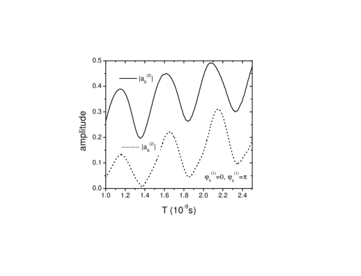
FIG. 1.: Amplitudes $\left|a_{9}^{(2)}\right|$ and $\left|a_{8}^{(2)}\right|$ as a function of pulse duration $T$ (for $\varphi_{9}^{(1)}=0$ and $\varphi_{8}^{(1)}=\pi$)

The work is supported by the National Natural Science Foundation of China, Shanghai Research Center of Applied Physics, Institute of Physics of Chinese Academy of Sciences, and a CRCG grant of the University of Hong Kong.

^†E-mail: rbtao@fudan.ac.cn

REFERENCES

[1] D. Deutsch, Proc. R. Soc. (London) Ser. A 400, 97
(1985)
[2] L. K. Grover, Phys. Rev. Lett. 79, 325 (1997)
[3] L. K. Grover, Phys. Rev. Lett. 79, 4709 (1997)
[4] J. Ahn, T. C. Weinacht, and P. H. Bucksbaum, Science 287, 463 (2000)
[5] M. N. Leuenberger and D. Loss, Nature 410, 789
(2001)
[6] A. L. Barra, D. Gatteschi, and R. Sessoli, Phys. Rev. B
56, 8192 (1997)