Anisotropies of the Hamiltonian and the Wave Function: Inversion Phenomena in Quantum Spin Chains

1 Introduction

In the ground state problem of the antiferromagnetic quantum spin chains with the $XXZ$ interaction anisotropy $\mathchar 28929\relax\equiv J_{z}/J_{\perp}$, the Ising-like anisotropy $\mathchar 28929\relax>1$ is usually favorable to the Néel state and the $XY$-like anisotropy $\mathchar 28929\relax<1$ to the spin-fluid (SF) state. This can be seen, for instance, in the $S=1/2$ $XXZ$ chain and the $S=1$ $XXZ$ chain, although the Haldane phase exists between the Néel and the SF phase for the latter case. Very recently we have found that the inversion phenomenon between the anisotropies of the interaction and the wave function.[1] Namely, the SF state is realized for the Ising-like case and the Néel state for the $XY$-like case in the $S=1/2$ distorted diamond spin chain[2] with the $XXZ$ anisotropy. This inversion phenomenon is considered to be due to the interplay among the frustration, the trimer nature and the $XXZ$ anisotropy of the Hamiltonian. In case of strong frustrations, the spin system tends to form singlet pairs to avoid the energy loss by competing interactions [3]. But the formation of singlet pairs is incompatible with the trimer nature. Thus, in the $XY$-like anisotropy case, the spins turn to the $z$-direction to avoid the energy loss, because interaction of the $z$-direction is weaker than that of the $xy$-direction in the $XY$-like case. Similarly, we can explain the existence of the SF state for the Ising-like anisotropy case.

If this physical explanation is to the point, the inversion phenomenon will be observed in many quantum spin chain models having the frustration, the trimer nature and the $XXZ$ anisotropy. From this point of view, we have investigated the $S=1/2$ trimerized $XXZ$ chain with the next-nearest-neighbor interactions, which may be the most fundamental model with these three characteristics.

2 $S=1/2$ Trimerized ${\mbox{\boldmath$X$}XZ}$ Spin Chain with Next-Nearest-Neighbor Interactions

Our model is the $S=1/2$ trimerized $XXZ$ chain with the next-nearest-neighbor interactions (Fig. 1), having the Hamiltonian

$$H=J_{1}\sum_{i}\{h_{3i-1,3i}(\mathchar 28929\relax)+h_{3i,3i+1}(\mathchar 28929\relax)\}+J_{2}\sum_{i}h_{3i-2,3i-1}(\mathchar 28929\relax)+J_{3}\sum_{j}h_{j,j+2}(\mathchar 28929\relax),$$ (2.1)

where

$$h_{m,n}\equiv S_{m}^{x}S_{n}^{x}+S_{m}^{y}S_{n}^{y}+\mathchar 28929\relax S_{m}^{z}S_{n}^{z}.$$ (2.2)

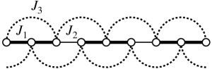
Fig. 1: The $S=1/2$ trimerized $XXZ$ chain with the next-nearest-neighbor interactions.

The quantity $J_{1}$ (thick lines) denotes the intra-trimer nearest-neighbor coupling, $J_{2}$ (thin lines) the inter-trimer nearest-neighbor coupling and $J_{3}$ (broken lines) the next-nearest-neighbor coupling. All the couplings are assumed to be positive (antiferromagnetic). Hereafter we focus on the $J_{1}\gg J_{2},J_{3}$ case for simplicity, where the inversion phenomenon was observed in the on $S=1/2$ distorted diamond chain with $XXZ$ anisotropy.

Let us discuss the ground state of our model by use of the degenerate perturbation theory. First we consider the 3-spin problem of ${\mbox{\boldmath$S$}}_{3i-1},{\mbox{\boldmath$S$}}_{3i}$ and ${\mbox{\boldmath$S$}}_{3i+1}$. As far as $J_{1}\gg J_{3}$, the ground states of the 3-spin cluster are

$$|\Uparrow_{i}\rangle\equiv{1\over A}(|\uparrow\uparrow\downarrow\rangle-a|\uparrow\downarrow\uparrow\rangle+|\downarrow\uparrow\uparrow\rangle)$$ (2.3)

$$|\Downarrow_{i}\rangle\equiv{1\over A}(|\uparrow\uparrow\downarrow\rangle-a|\uparrow\downarrow\uparrow\rangle+|\downarrow\uparrow\uparrow\rangle)$$ (2.4)

where $|\uparrow\uparrow\downarrow\rangle$ means $|\uparrow_{3i-1}\uparrow_{3i}\downarrow_{3i+1}\rangle$ for instance, $A=\sqrt{2+a^{2}}$ and

$$a={-3\tilde{J}_{3}+\mathchar 28929\relax+r\over 2+\tilde{J}_{3}^{2}+\tilde{J}_{3}\mathchar 28929\relax-J_{3}r},~{}~{}~{}~{}~{}r=\sqrt{8+(\tilde{J}_{3}+\mathchar 28929\relax)^{2}}$$ (2.5)

where $\tilde{J}_{3}\equiv J_{3}/J_{1}$. As far as $J_{1}\gg J_{2},J_{3}$, we can restrict ourselves to these two states, $|\Uparrow_{j}\rangle$ and $|\Downarrow_{j}\rangle$, for the $j$th trimer, neglecting other 6 states. For convenience we consider $|\Uparrow_{j}\rangle$ and $|\Downarrow_{j}\rangle$ as the up-spin and down-spin states of the pseudo-spin ${\mbox{\boldmath$T$}}_{j}$, respectively. The interactions between the trimers are expressed as the interactions between pseudo-spins. For instance, we have

$${J_{3}\over 2}\left(S_{3j}^{+}S_{3j+2}^{-}+S_{3j}^{-}S_{3j+2}^{+}\right)\Rightarrow-{2aJ_{3}\over(a^{2}+2)^{2}}\left(T_{j}^{+}T_{j+1}^{-}+T_{j}^{-}T_{j+1}^{+}\right)$$ (2.6)

In the lowest order with respect to $J_{2}$ and $J_{3}$, a straightforward calculation leads to

$$H_{\rm eff}=\sum_{j}\left\{J_{\rm eff}^{\perp}\left(T_{j}^{x}T_{j+1}^{x}+T_{j}^{y}T_{j+1}^{y}\right)+J_{\rm eff}^{z}T_{j}^{z}T_{j+1}^{z}\right\}$$ (2.7)

where

$$J_{\rm eff}^{\perp}={a\over(a^{2}+2)^{2}}\left\{4aJ_{2}-8J_{3}\right\}$$ (2.8)

$$J_{\rm eff}^{z}={a\over(a^{2}+2)^{2}}\left\{a^{2}(a^{2}-2)J_{2}-2(a^{2}-2)^{2}J_{3})\right\}$$ (2.9)

In the effective theory of the lowest order with respect to $J_{2}/J_{1}$ and $J_{3}/J_{3}$, we can let $J_{3}=0$ in $a$, that is

$$a={\mathchar 28929\relax+\sqrt{\mathchar 28929\relax^{2}+8}\over 2}$$ (2.10)

When $\mathchar 28929\relax=1$, we see $J_{\rm eff}^{\perp}=J_{\rm eff}^{z}=(4/9)(J_{2}-J_{3})$. Then the ground state of $H_{\rm eff}$ is either the ferromagnetic state or the spin-fluid state depending on whether $J_{2}<J_{3}$ or $J_{2}>J_{3}$. The ferromagnetic state of the $T$-system corresponds to the ferrimagnetic state of the $S$-system with the magnetization of $M_{\rm s}/3$, where $M_{\rm s}$ is the saturation magnetization.

In general case ($\mathchar 28929\relax\neq 1$), the ground state of $H_{\rm eff}$ is known from $J_{\rm eff}^{\perp}$ and $J_{\rm eff}^{z}$ as

$$\matrix{J_{\rm eff}^{z}<0\hbox{ and }|J_{\rm eff}^{z}|>|J_{\rm eff}^{\perp}|&~{}~{}\Rightarrow~{}~{}&\hbox{ferromagnetic state}\hfill\cr|J_{\rm eff}^{z}|<|J_{\rm eff}^{\perp}|\hfill&~{}~{}\Rightarrow~{}~{}&\hbox{spin-fluid state}\hfill\cr J_{\rm eff}^{z}>|J_{\rm eff}^{\perp}|\hfill&~{}~{}\Rightarrow~{}~{}&\hbox{N\'{e}el state}\hfill}$$ (2.11)

which leads to

$$\matrix{&&\hbox{$XY$-like}&\hbox{Ising-like}\cr J_{3}<c_{1}J_{2}&&\hbox{SF}&\hbox{N\'{e}el }\cr c_{1}J_{2}<J_{3}<c_{2}J_{2}&&\hbox{N\'{e}el}&\hbox{SF}\cr J_{3}>c_{2}J_{2}&&\hbox{SF}&\hbox{ferro}}$$ (2.12)

where

$$c_{1}={a^{2}+2a+2\over 2a(a+2)}~{}~{}~{}~{}~{}~{}~{}c_{2}={1\over 2}{a(a+2)(a^{2}-2a+2)\over a^{4}-4a^{2}+8}$$ (2.13)

We note that

$$c_{1}\to 5/8~{}~{}~{}~{}~{}c_{2}\to 1~{}~{}~{}~{}~{}(\hbox{as }\mathchar 28929\relax\to 1)$$ (2.14)

The phase diagrams for the $\mathchar 28929\relax=1,\ 0.5\mbox{~{}and~{}}2.5$ cases near the truncation point $J_{2}=J_{3}=0$ are shown in Figs. 2-4, where $\tilde{J}_{2}\equiv J_{2}/J_{1},\ \tilde{J}_{3}\equiv J_{3}/J_{1}$.

Fig. 2: Phase diagram for the $\mathchar 28929\relax=1$ case.

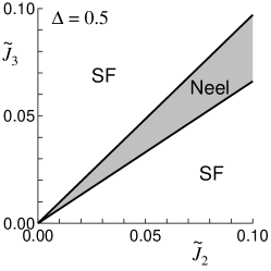
Fig. 3: Phase diagram for the $\mathchar 28929\relax=0.5$ case.

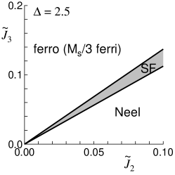
Fig. 4: Phase diagram for the $\mathchar 28929\relax=2.5$ case.

In the Ising limit $\mathchar 28929\relax\to\infty$, we see $c_{1}=c_{2}=1/2$, resulting in the vanishing of the spin-fluid state in Fig. 4. The remarkable nature of Fig. 3 is the existence of the Néel region, although the interaction anisotropy is $XY$-like. Similarly, the SF state is realized in Fig. 4 in spite of the Ising-like anisotropy. These are the inversion phases.

We have also performed the numerical diagonalization by use of the Lanczös method and analyzed the numerical data by the level spectroscopy method.[4, 3, 6, 7] For instance, when $\tilde{J}_{2}=0.01$ and $\mathchar 28929\relax=0.5$, the critical values of the SF-Néel transitions are $(\tilde{J}_{3})_{\rm cr1}=0.006610$ and $(\tilde{J}_{3})_{\rm cr2}=0.009696$, showing good agreements with the theoretical values from Eqs.(2.12) and (2.13) $(\tilde{J}_{3})_{\rm cr1}=0.006609$ and $(\tilde{J}_{3})_{\rm cr2}=0.009703$, respectively. For the $\tilde{J}_{2}=0.01$ and $\mathchar 28929\relax=2.5$ case, we have obtained $(\tilde{J}_{3})_{\rm cr1}=0.005623$ (Néel-SF) and $(\tilde{J}_{3})_{\rm cr2}=0.006863$ (SF-ferrimagnetic), also having good agreements with the theoretical values $(\tilde{J}_{3})_{\rm cr1}=0.006609$ and $(\tilde{J}_{3})_{\rm cr2}=0.006850$, respectively.

3 Concluding Remarks

We have shown that there exist inversion regions in the $S=1/2$ trimerized $XXZ$ chain with next-nearest-neighbor interactions by use of the degenerate perturbation theory as well as the level spectroscopy analysis[4] of the numerical data obtained by the Lanczös method. This strongly suggests that the inversion phenomenon is popular to the $=1/2$ $XXZ$ models with the frustration and the trimer nature. In fact, this phenomenon has been also found in the $S=1/2$ frustrated 3-leg ladder with the $XXZ$ anisotropy.[5]

In this paper we have restricted ourselves to the $J_{1}\gg J_{2},J_{3}$ case for simplicity. In case of larger $J_{3}$, the dimer ground state is expected. In fact, when $J_{2}=J_{1}$, our model is reduced to the uniform $XXZ$ chain with next-nearest-neighbor interactions, which shows the SF-dimer or Néel-dimer transitions.[3, 6, 7] The full phase diagram of the present model will be reported elsewhere.

References

[1]
K. Okamoto and Y. Ichikawa,
to be published in J. Phys. Chem. Solids,
cond-mat/0108528.
[2]
K. Okamoto, T. Tonegawa, Y .Takahashi and M .Kaburagi:
J. Phys.: Cond. Matter 11 (1999), 10485.
[3]
K. Okamoto and K. Nomura,
Phys. Lett. A169 (1992), 433
and refereces therein.
[4]
K. Okamoto,
Prog. Theor. Phys. in this issue.
[5]
K. Okamoto and T. Sakai,
in preparation.
[6]
K. Nomura and K. Okamoto,
J. Phys. Soc. Jpn. 62 (1993), 1123.
[7]
K. Nomura and K. Okamoto,
J. Phys. A: Math. Gen. 27 (1994), 5773.