Exact ground state of the generalized three-dimensional Shastry-Sutherland model

Abstract

We generalize the Shastry-Sutherland model to three dimensions. By representing the model as a sum of the semidefinite positive projection operators, we exactly prove that the model has exact dimer ground state. Several schemes for constructing the three-dimensional Shastry-Sutherland model are proposed.

PACS numbers: 75.10.Jm

There has been an increasing interest in the Shastry-Sutherland (S-S) model[1] since it can describe many aspects of the two-dimensional spin gap system $SrCu_{2}(BO_{3})_{2}$.[2, 3] In a series of theoretical investigations, various aspects of the S-S model have been described. [4, 5, 6, 7, 8]

The S-S model is a two dimensional square lattice antiferromagnet with additional diagonal interactions in every second square with alternating directions, see Fig. 1. For the square lattice interaction $J$ and the diagonal interaction $J_{d}$, the Hamiltonian can be written as

$$H=J\sum_{\langle i,j\rangle}{\bf S}_{i}\cdot{\bf S}_{j}+J_{d}\sum_{\langle i,j\rangle_{d}}{\bf S}_{i}\cdot{\bf S}_{j}$$ (1)

Shastry and Sutherland have shown that the product of singlet pairs (dimers) along the diagonal bonds is the ground state of the system for $J_{d}\geq 2J$.

FIG. 1.: The Sharstry-Sutherland lattice.

In this paper we generalize the S-S model to three dimensions with various types of interactions. Between the different planes we can construct the exact ground states of three-dimensional models and by this increase the number of three-dimensional models with the exactly known ground states. We consider a three-dimensional cubic lattice (Fig.2) constructed from basic cubic units shown in Fig.3. Each layer in this cubic system is a S-S lattice which is coupled to the next layer by the perpendicular interlayer interaction $J_{\perp}$ and the diagonal interaction $J_{\times}$ connected the diagonal end points to those in the next layer. That means that the Sharstry-Sutherland diagonals are on top of each other. If we label the different layers by $\alpha=1,\cdots,L$ and have $N\times M$ sites per layer, the Hamiltonian can be written as

$$H = J\sum_{\langle i,j\rangle,\alpha}{\bf S}_{i}^{\alpha}\cdot{\bf S}_{j}^{\alpha}+J_{d}\sum_{\langle i,j\rangle_{d},\alpha}{\bf S}_{i}^{\alpha}\cdot{\bf S}_{j}^{\alpha}$$ (2)

$$+ J_{\times}\sum_{\langle i,j\rangle_{d^{\prime}},\alpha}\left({\bf S}_{i}^{\alpha}\cdot{\bf S}_{j}^{\alpha+1}+{\bf S}_{j}^{\alpha}\cdot{\bf S}_{i}^{\alpha+1}\right)$$ (3)

$$+ J_{\perp}\sum_{i,\alpha}{\bf S}_{i}^{\alpha}\cdot{\bf S}_{i}^{\alpha+1}\;,$$ (4)

Periodic boundaries in each layer are assumed and $M$ and $N$ have to be even, while $L$ can be even or odd.

FIG. 2.: The generalized 3D Sharstry-Sutherland model.

It is instructive to consider two different parameter limits of our model (4): (i) For $J_{\perp}=J_{\times}=0$, the 3D model reduces to $L$ independent S-S layers. (ii) For $J=0$ within each layer, the three-dimensional system decouples to independent $\frac{1}{2}N\times M$ two-leg spin ladders of length $L$. The structure of this ladder is shown in Fig.4 (a). It is known that such a spin ladder with $J_{\perp}=J_{\times}$ has exact ground state composed of a product of dimers along the rungs of ladder [10] as long as the exchange interaction along the rung satisfies the condition $J_{d}\geq 2J_{\perp}$. This means that in both of the special cases, the product of singlet pairs along the inlayer diagonal bonds is the exact ground state of the model (4). In the following, we will prove that for the general case (but $J_{\perp}=J_{\times}$) the ground state of the three-dimensional model is given by the product of all diagonal singlet pairs

$$\Phi_{D}=\prod_{\alpha=1}^{L}\prod_{\langle i,j\rangle_{d}}\frac{1}{\sqrt{2}}\left([\uparrow]_{i}^{\alpha}[\downarrow]_{j}^{\alpha}-[\downarrow]_{i}^{\alpha}[\uparrow]_{j}^{\alpha}\right)$$ (5)

for special condition

$$J_{d}\geq 2(J+J_{\perp})$$ (6)

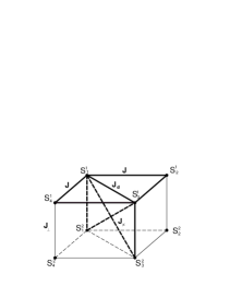
FIG. 3.: The basic cubic unit with inlayer and interlayer diagonal exchange interactions which constructs the 3D Sharstry-Sutherland model. (See text for further discussion)

The rigorous proof is made by representing the above model as a sum of the positive semidefinite projection operators and the above condition (6) guarantees that $\Phi_{D}$ is the ground state of the system. The proof furthermore employs the fact that the global Hamiltonian (4) can be written as a sum of many local sub-Hamiltonians defined on the basic cubic unit (see Fig.3). There are altogether $Q=\frac{1}{2}N\times M\times L$ units as local sub-Hamiltonians $h$. This part of the Hamiltonian can be written as

$$h = J_{d}{\bf S}_{1}^{1}\cdot{\bf S}_{3}^{1}+J({\bf S}_{1}^{1}+{\bf S}_{3}^{1})\cdot({\bf S}_{2}^{1}+{\bf S}_{4}^{1})$$ (7)

$$+ J_{\perp}({\bf S}_{1}^{1}+{\bf S}_{3}^{1})\cdot({\bf S}_{1}^{2}+{\bf S}_{3}^{2}),$$ (8)

which is just the sum of spin exchange interactions along the bonds represented by bold lines in Fig. 3. Those spin interactions represented by thin lines belong to the neighboring cubes.

We now define a projection operator ${\bf P}$ composed of three one half spins as

$${\bf P}[{\bf S}_{1},{\bf S}_{2},{\bf S}_{3}]=\frac{1}{3}\left[\left({\bf S}_{1}+{\bf S}_{2}+{\bf S}_{3}\right)^{2}-\frac{3}{4}\right],$$ (9)

which projects a state into the subspace with total spin $3/2$. Using the projection operators, we can transform our Hamiltonian part $h$ which is represented as

$$h = -\frac{3}{4}(2J+2J_{\perp})+(J_{d}-2J-2J_{\perp}){\bf S}_{1}^{1}\cdot{\bf S}_{3}^{1}$$ (12)

$$+J~{}~{}\left[{\bf P}({\bf S}^{1}_{1},{\bf S}^{1}_{2},{\bf S}^{1}_{3})+{\bf P}({\bf S}^{1}_{1},{\bf S}^{1}_{4},{\bf S}^{1}_{3})\right]$$

$$+J_{\perp}\left[{\bf P}({\bf S}^{1}_{3},{\bf S}^{1}_{1},{\bf S}^{2}_{1})+{\bf P}({\bf S}^{1}_{1},{\bf S}^{1}_{3},{\bf S}^{2}_{3})\right]\;.$$

It is obvious that, for $J_{d}=2(J+J_{\perp})$, certain terms in Eq. (12) vanish and thereby the Hamiltonian is a sum of four positive semidefinite projection operators. The singlet state

$$\left[{\bf S}^{1}_{1},{\bf S}^{1}_{3}\right]=\left([\uparrow]_{1}^{1}[\downarrow]_{3}^{1}-[\downarrow]_{1}^{1}[\uparrow]_{3}^{1}\right)/\sqrt{2}$$ (13)

has the lowest eigenvalue $0$ for each of the four projection operators and thus is the ground state of this sub-Hamiltonian. For larger $J_{d}$ this singlet is also the lowest energy eigenstate of the term ${\bf S}_{1}^{1}\cdot{\bf S}_{3}^{1}$, and hence it is the ground state of the total sub-Hamiltonian $h$ with the ground state energy $E_{h}=-\frac{3}{4}J_{d}$. All the other sub-Hamiltonians defined on other basic units of cube have the same properties as the one explicitly shown in Fig. 3. Therefore, the global ground state of this three-dimensional model is just a product of dimers for each layer. Such a ground state is essentially an optimum ground state of the global Hamiltonian, since it is simultaneously ground state of every local sub-Hamiltonian.[9] The corresponding ground state energy is then given by

$$E=-\frac{3}{4}QJ_{d}.$$ (14)

FIG. 4.: The spin ladders correspond to the 3D S-S model with $J=0$.

This general proof actually does not depend on the special coupling parameters between the layers we discussed so far. We see that the main condition is that the dimer along the diagonals in the layer should be also the dimers along the rungs of the corresponding ladders. And as long as the vertical spin ladders have dimers along the rungs as ground states, we can put them together in three dimensions. Therefore, generalization of the model (4) is straightforward by changing the inter-layer coupling way. The first example is that we couple the different layers only along one interlayer diagonal (Fig.4. (b)). In this case we require $J_{\times}=2J_{\perp}$ which means that the individual ladders are Majumdar-Gosh chains.[11] The second example is given when the two legs of ladder have different interactions (Fig. 4. (c)).[12, 13] If we call them $J_{\perp}$ and $J^{\prime}_{\perp}$, we should have the conditions

$$J_{\times}=J_{\perp}+J^{\prime}_{\perp}$$ (15)

and

$$J_{d}\geq 2J+J_{\perp}+J^{\prime}_{\perp}.$$ (16)

Even the limit $J^{\prime}_{\perp}=0$ is allowed and we have vertical sawtooth chains coupled together. [14, 15] In the third example, we may couple the different layers by some intermediate spins shown in Fig.5. If this coupling has a strength $J^{\prime}$, we should have the condition

$$J_{d}\geq 2J+J^{\prime}$$ (17)

and the ground state is still a product of dimers each layer. There could be of course other constructions. The main point is that we have shown that the Shastry-Sutherland layer could be coupled to other layers by different mechanisms which only have to make sure that these ladders have dimers on the rungs as ground state.

FIG. 5.: The dimers on neighboring layers (rungs) have no direct coupling, but couple to an intermediate spin between them with exchange strength of $J^{\prime}$.

We have limited our discussion to homogeneous models in which every basic unit has the same structure and exchange strength. We can also generalize our discussion to inhomogeneous cases, e.g. to a model where the inlayer coupling strengths, $J^{\alpha}$ and $J^{\alpha}_{d}$, are different in each layer. In this case we only have to make sure that the constraint

$$J^{\alpha}_{d}\geq 2(J^{\alpha}+J_{\perp})$$ (18)

is still fulfilled.

To conclude, we extend the two dimensional S-S model to three dimension and find the exact ground state of the generalized three-dimensional S-S model. An exact proof based upon the representation of projection operators is given. We also discuss several ways of extending the 3D S-S model.

S. Chen would like to specially thank J. Voit for his critical reading of the manuscript and encouragement. This research was supported by DFG through Grants No. VO436/7-2.

REFERENCES

- [1] B. S. Shastry and B. Sutherland, Physica B 108, 1069 (1981).
- [2] H. Kageyama et al., Phys. Rev. Lett. 82, 3168(1999).
- [3] S. Miyahara and K. Ueda, Phys. Rev. Lett. 82, 3701(1999).
- [4] C. H. Chung, J. B. Marston, and S. Sachdev, Phys. Rev. B. 64, 134407 (2001).
- [5] W. Zheng, J. Oitmaa and C.J. Hamer, cond-mat/0107019.
- [6] D. Carpentier and L. Balents, cond-mat/0102218.
- [7] K. Totsuka, S. Miyahara and K. Ueda, Phys. Rev. Lett. 86, 520 (2001).
- [8] G. Misguich, Th. Jolicoeur and S. M. Girvin, Phys. Rev. Lett. 87, 097203 (2001).
- [9] H. Niggemann and J. Zittartz, Z. Phys. B. 101, 289 (1996).
- [10] I. Bose and S. Gayen, Phys. Rev. B. 48, 10653 (1993).
- [11] C. K. Majumdar and D. K. Ghosh, J. Math. Phys. 10, 1388 (1969); 10, 1399 (1969). (1982); 26, 5257 (1982)
- [12] S. Chen, H. Büttner and J. Voit, Phys. Rev. Lett. 87, 087205 (2001).
- [13] S. Chen, H. Büttner and J. Voit, (unpublised).
- [14] D. Sen, B. S. Shastry, R. E. Walstedt and R. Cava, Phys. Rev. B. 53, 6401 (1996).
- [15] T. Nakamura and K. Kubo, Phys. Rev. B. 53, 6393 (1996).