Shot Noise in Schottky’s Vacuum Tube is Classical

Abstract

In these notes we discuss the origin of shot noise (’Schroteffekt’) of vacuum tubes in detail. It will be shown that shot noise observed in vacuum tubes and first described by W. Schottky in 1918 [1] is a purely classical phenomenon. This is in pronounced contrast to shot noise investigated in mesoscopic conductors [2] which occurs due to quantum mechanical diffraction of the electronic wave function.

84.47+w, 72.70.+m

]

I Introduction

Shot noise is due to time-dependent fluctuations in the electrical current caused by the random transfer of discrete units of charge. In 1918 Schottky [1] analyzed these fluctuations in vacuum tubes theoretically for the first time arriving at his famous Schottky formula. It states that the spectral density $S$ of the fluctuations at ‘low’ frequencies is proportional to the unit of charge $e$ and to the mean electrical current $|I|$.

In recent years shot noise of mesoscopic conductors has been investigated extensively [2]. In these systems shot noise is a $quantum$ phenomenon originating from the diffraction of wave functions [3]. It is the quantum mechanical uncertainty of not knowing with absolute certainty whether a particle incident on a scattering region transmit from source to drain that is responsible for shot noise. Schottky derived his formula before the existence of quantum mechanics, solely making use of classical statistical mechanics. In retrospect one may ask the question whether shot noise in the vacuum tube is classical or not. The answer is not straightforward as many discussions with colleagues have shown. Most engineers, for example, are convinced that shot noise is a classical phenomenon altogether. The mesoscopic physics community, on the other hand, tend to believe that shot noise in electrical conductor is quantum in general. There are colleagues who are in favor of a quantum-mechanical origin for shot noise observed in the vacuum tube. This has motivated us to analyze the randomness contributing to shot noise in vacuum tubes in detail. It turns out that quantum diffraction in the emission process can be neglected in vacuum tubes. The main source of noise stems from the the $classical$ occupation of electron states (i.e. the Boltzmann tail) within the cathode. Hence, Schottky’s vacuum tube is classical!

II Shot noise of a two-terminal conductor

We start with a simple derivation of the expression for the power spectral density of the noise of a two-terminal conductor along the lines of Martin and Landauer [4]. In their paper the fluctuating currents are a result of the random transmission of electrons from one terminal to the other. Different processes contribute to the noise for each energy $E$ and mode $n$ (only elastic scattering is assumed):

1. A current pulse occurs whenever an electron wave packet incident from the left terminal (source) is scattered into an empty state in the right terminal (drain). The rate $\tau_{rl}^{-1}$ of these events is proportional to the probability $f_{L}(E)$ that an energy state $E$ in the left reservoir is occupied, times the probability $1-f_{R}(E)$ that a respective state in the right reservoir is unoccupied, times the transmission probability from left to right: $T_{n}^{rl}(E)\equiv T_{n}(E)$:

   $$\tau_{rl}^{-1}\sim f_{L}(E)[1-f_{R}(E)]\,T_{n}(E).$$ (1)

2. Of course the reverse process that electrons scatter from an occupied state in the right reservoir to an unoccupied state in the left reservoir contributes to noise, too. The rate of these processes is given by:

   $$\tau_{lr}^{-1}\sim f_{R}(E)[1-f_{L}(E)]\,T_{n}(E),$$ (2)

   where $T_{n}^{lr}(E)=T_{n}^{rl}(E)\equiv T_{n}(E)$ has been taken into account.

Since we require an expression for the fluctuations, i.e. the deviations from the mean current, the mean current squared has to be subtracted. As the current is proportional to to $T_{n}(E)\,[f_{L}(E)-f_{R}(E)]$, the contribution from electrons at energy $E$ in one specific mode $n$ to the noise is proportional to:

$$f_{L}(E)[1-f_{R}(E)]\,T_{n}(E)+f_{R}(E)[1-f_{L}(E)]\,T_{n}(E)\rule[-5.69054pt]{0.0pt}{14.22636pt}$$ (3)

$$\hskip 51.21495pt-\,[f_{L}(E)-f_{R}(E)]^{2}\,T_{n}^{2}(E).$$ (4)

The coefficient follows from the fact that if no bias is applied ($V=0$) the expression for thermal noise $4k_{B}\theta G$ must be recovered ($\theta$ is the temperature):

$$S = 4k_{B}\theta G\;=\;4k_{B}\theta\,G_{0}\int dE\,\left(-\frac{\partial f}{\partial E}\right)\sum_{n}T_{n}(E)$$ (5)

$$= 2G_{0}\sum_{n}\int dE\,2f(E)[1-f(E)]T_{n}(E),$$ (6)

with $G_{0}=2e^{2}/h$. In equilibrium ($V=0$), $f_{L}(E)=f_{R}(E)\equiv f(E)$, where $f$ denotes the Fermi-Dirac distribution. Then, expression (4) equals

$$2f(E)[1-f(E)]\,T_{n}(E).$$ (7)

Comparing Eq. (6) and Eq. (7) the general expression for the shot noise of a two-terminal conductor (in the zero frequency limit) follows as [5, 6]:

$$S = 2\,G_{0}\sum_{n}\int dE\,\{f_{L}(1-f_{R})\,T_{n}+f_{R}(1-f_{L})\,T_{n}$$ (9)

$$-\,[f_{L}-f_{R}]^{2}\,T_{n}^{2}\}$$

$$= 2\,G_{0}\sum_{n}\int dE\,\{[f_{L}(1-f_{R})+f_{R}(1-f_{L})]\,T_{n}(1-T_{n})$$ (11)

$$+\,[f_{L}(1-f_{L})+f_{R}(1-f_{R})]^{2}\,T_{n}^{2}\}$$

III Vacuum tubes

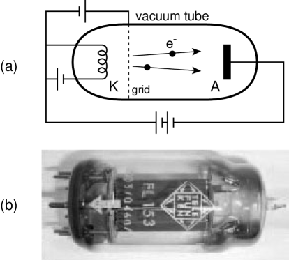
FIG. 1.: Vacuum tubes: (a) Schematics of a triode. Electrons having enegies larger than the work function $W$ of the tungsten filament are emitted from the heated cathode (K), travel through the vacuum and are attracted by the positive anode (A). (b) Photograph of a historical tetrode (triode with additional grid) containing 4 electrodes (Telefunken EL 153).

Figure 1(a) shows a schematics of a vacuum tube (triode): The heated cathode (K) made of a wounded tungsten wire boils off electrons into the vacuum. The emitted elctrons are attracted by the positively charged anode (Edison effect). A negatively biased grid (or many grids) between cathode and anode controls the electron current. By designing the cathode, grid(s) and plate properly, the tube converts a small AC voltage at the grid into a larger AC signal, thus amplifying it [7]. In the following we diregard the grid and consider only the vacuum diode (as Schottky did).

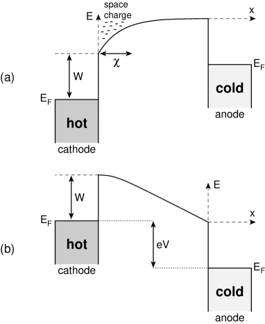
FIG. 2.: (a) Space-charge region formed in front of the cathode in a open-circuited tube. (b) For sufficiently high bias voltages $V$ the space-charge is removed (saturation regime) and the potential drops linearly. $W$ denotes the work function.

If the anode is floating, no net current flows from cathode to anode [Fig. 2(a)]. Instead, a negative space-charge is formed in front of the cathode, originating from evaporated electrons which are hold back by the ionized atoms. The size $\chi$ of the space-charge region can be calculated solving the Poisson-equation $\Delta\varphi(x)=-en(x)/\epsilon_{0}$ for the electrical potential $\varphi(x)$ with the electron density $n(x)=n_{0}\exp(-e\varphi(x)/k_{B}\theta)\simeq n_{0}\,[1-e\varphi(x)/k_{B}\theta]$, where $n_{0}$ is the electron densitiy within the cathode:

$$\chi=\sqrt{\frac{\epsilon_{0}k_{B}\theta}{n_{0}e^{2}}}.$$ (12)

The higher the temperature $\theta$ the larger the space-charge region.

On the other hand, if the circuit is closed and the cathode is kept at an elevated temperature, a thermionic current flows from cathode to anode [Fig. 2(b)]. The magnitude of this current is limited by the negative space-charge region in front of the cathode. This is also true if the anode is kept at a moderate positive potential. In this space-charge limited regime, the magnitude of the current is given by:

$$I=\frac{\sqrt{2}}{9\pi}\sqrt{\frac{e}{m}}\frac{V^{3/2}}{L^{2}}$$ (13)

with $L$ the distance between cathode and anode [7]. Only for sufficiently large bias voltages $V$ are all emitted electrons attracted by the anode and the space-charge region is removed. In this case, the current saturates (does no longer depend on the anode voltage) and is determined by the temperature of the cathode [Fig. 3].

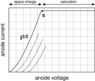
FIG. 3.: Current-voltage characteristics of a vacuum tube illustrating the 3/2-power law [Eq. (13)] and the saturation point (S). The dashed curves are IV-curves for different grid voltages. Within the saturation regime the current does no longer depend on the anode voltage because all electrons emitted by the cathode are collected at the anode.

In the space-charge limited regime where the possibility of escape of an electron is limited by Coulomb repulsion shot noise is suppressed. Full shot noise $S=S_{Poisson}=2e|I|$ is only present in the saturation regime [8]. The question whether shot noise in the saturation regime is classical or quantum in nature will be discussed in sect. V. Before, the electrical field and current in the saturation regime will be estimated.

IV Electrical field and current in the saturation regime

At the edge of the vacuum barrier the electron density is approximatively given by $n_{0}=a^{-3}\,\exp(-W/k_{B}\theta)\simeq 5\cdot 10^{16}$ m³ with $a\simeq 1.2$ $\AA$ the typical interatomic distance, $W=4.5$ eV the work function of tungsten and $\theta=$ 2000 K the cathode temperature. The size $\chi$ of the space-charge region follows from (12) and is of the order 10 $\mu$m. The charge build up at the cathode corresponds to an electrostatic surface potential of $k_{B}\theta/e$, so that the surface electric field can be estimated as $\mbox{$\cal{E}$}\simeq k_{B}\theta/e\chi$. Inserting numbers the saturation field is of the order $10^{4}$ V/m.

The electrical current density due to thermionic emission from a heated conductor is given by the Richardson-Dushman equation [9]:

$$j=\mbox{$\cal{L}$}\,\theta^{2}\exp(-W/k_{B}\theta)$$ (14)

with $\mbox{$\cal{L}$}=emk_{B}^{2}/2\pi^{2}\hbar^{3}=120$ AK^-2cm^-2. This expression is only correct if the electrical field $\cal{E}$ is so high that the space-charge region is removed (saturation regime).

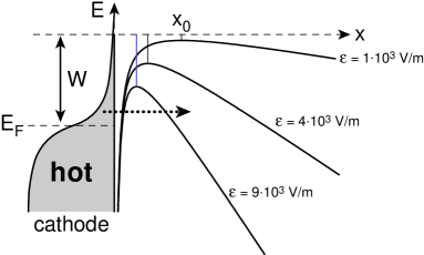
FIG. 4.: Image potential determining the barrier shape in emission of electrons from the hot cathode for different electrical fields $\cal{E}$. For very high fields the barrier becomes very thin allowing for electrons to tunnel (quantum regime).

An emitting electron experiences a potential $\phi$ determined by the saturation field $\cal{E}$ and its image potential in the (planar) cathode (image-potential), Fig. 4:

$$\phi(x)=-\mbox{$\cal{E}$}x-\frac{e}{4\pi\epsilon_{0}}\frac{1}{x}$$ (15)

The maximum of $\phi(x)$ lies at $x_{0}=\sqrt{e/4\pi\epsilon_{0}\mbox{$\cal{E}$}}$, where the barrier is lowered by $e\phi(x_{0})=-2e\sqrt{e\mbox{$\cal{E}$}/4\pi\epsilon_{0}}\simeq-8$ meV. This is negligible in comparison with the work function $W=4.5$ eV, so that the saturation current can be estimated disregarding the barrier lowering. For a cathode area of 10^-2 cm^-2 and $\theta=2000$ K the emission current is of the order 10 $\mu$A.

V The ‘Schroteffekt’ in vacuum tubes

In the saturation regime (no space-charge at the cathode) the shot noise due to the emission of electrons from cathode to anode is according to Eq. (11) given by

$$S=2G_{0}\sum_{n}\int dE\,\{\underbrace{f_{cathode}T_{n}(1-T_{n})}_{quantum}+\underbrace{f_{cathode}\,T_{n}^{2}}_{classical}\}.$$ (16)

Here we made use of the fact that $f_{R}=f_{anode}=0$ and that the occupation of states within the hot cathode at energy $W$ above $E_{F}$ is small (classical): $f_{L}=f_{cathode}=\exp(-W/k_{B}\theta)\ll 1$. Therefore, $f_{L}(1-f_{L})\simeq f_{L}$. The current $I$ due to emission at the cathode equals

$$I=\frac{2e}{h}\sum_{n}\int dE\,f_{cathode}\,T_{n}$$ (17)

There are two terms in Eq. (16) contributing to shot noise: the first term is of quantum mechanical origin since it only contributes for transmission probabilities $T\neq 0,1$, hence, only if there are quantum uncertainties. In contrast, the second term is classically because it dominates when all transmission coefficients are classical, i.e. either $0$ or $1$. As we show now, both classical and quantum parts may yield Schottky’s famous result independently.

Classical part: Because all $T_{n}$ are either $0$ or $1$, $T_{n}^{2}=T_{n}$ and shot noise is consequently given by

$$S=2G_{0}\sum_{n}\int dE\,f_{cathode}\,T_{n}.$$ (18)

With Eq. 17 we arrive at Schottky’s formula $S=2e|I|$.

Quantum part: In the special limit in which all $T_{n}$’s are small ($T_{n}\ll 1$) the noise is due to tunneling (quantum diffraction). In this case the quantum term $\sim T_{n}$ in Eq. (16) dominates, while terms proportional to $T_{n}^{2}$ are negligibly small. Hence again, $S$ is given by

$$S=2G_{0}\sum_{n}\int dE\,f_{cathode}\,T_{n}.$$ (19)

and we obtain Schottky’s formula $S=2e|I|$, this time however, originating from quantum diffraction.

In order to decide whether shot noise in vacuum tubes is classical or quantum, the transmission probabilities $T_{n}$’s need to be evaluated.

VI Transmission probability at the cathode

The quantum-mechanical transmission probability for electrons with energy $\epsilon$ above the barrier can be estimated with the following equation [10]:

$$T\simeq\left[1+e^{-2\pi\epsilon/\hbar\omega_{0}}\right]^{-1}$$ (20)

$\epsilon$ is of order $k_{B}\theta$ with $\theta$ the cathode temperature. $\omega_{0}$ denotes the negative curvature at the barrier top and determines whether the barrier is sharp or smooth. It can be obtained from the ‘force-constant’

$$f=e\left|\frac{\partial^{2}\varphi}{\partial x^{2}}\right|_{x=x_{0}}=2\sqrt{4\pi\epsilon_{0}e}\cdot\mbox{$\cal{E}$}^{3/2}$$ (21)

with $\omega_{0}=\sqrt{f/m}$ [11]:

$$\omega_{0}=\left(\frac{16\pi\epsilon_{0}e}{m^{2}}\right)^{1/4}\cdot\mbox{$\cal{E}$}^{3/4}.$$ (22)

If $\hbar\omega_{0}\ll k_{B}\theta$, $T=1$ and the classical part of the shot noise in (16) dominates. In the opposite limit $\hbar\omega_{0}\gg k_{B}\theta$, the transmission probability $T$ is small and shot noise is due to (quantum-mechanical) tunneling.

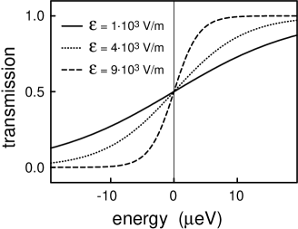
FIG. 5.: Transmission probability vs. energy $\epsilon$ according Eq. (20) for different saturation fields $\cal{E}$.

The first shot noise measurements in vacuum tubes were carried out by Hartmann in 1921 [12]. A very careful study of the ‘Schroteffekt’ was performed by Hull and Williams in 1925 [8]. In the first part of that latter experiment shot noise was measured in the saturation regime, where the thermionic current is limited by temperature [13]. The corresponding parameters are given in the first two lines of Tab. I. In this regime the full Schottky-noise $2e|I|$ has been measured in excellent agreement with Millikan’s value for the electron charge $e$. The ratio $\hbar\omega_{0}/k_{B}\theta\ll 1$, so that the transmission probability is $1$. Therefore, shot noise observed in this experiment is classical.

$\cal{E}$ [V/m]	$V_{G}$ [V]	$V_{P}$ [V]	$i_{0}$ [mA]	$\theta$ [K]	$\hbar\omega_{0}/k_{B}\theta$	T	$F$
$3\cdot 10^{6}$	120	120	1	1675	$3.2\,10^{-2}$	1	1.00
$3\cdot 10^{6}$	120	120	5	1940	$2.7\,10^{-2}$	1	1.00
$1\cdot 10^{4}$	-6	130	1	1675	$4.4\,10^{-4}$	1	0.93
$1\cdot 10^{4}$	-6	130	3	1805	$4.1\,10^{-4}$	1	0.49
$1\cdot 10^{4}$	-6	130	5	1940	$3.8\,10^{-4}$	1	0.20

TABLE I.: Experimental parameters from shot noise measurements of Hull and Williams in 1925. $V_{G}$ is the voltage at the grid and $V_{P}$ at the anode plate. $i_{0}$ is the thermionic current. $F=S/2e|I|$ denotes the Fano factor. The second last column shows that the shot noise observed in this experiment is a classical phenomenon.

In the second part of the experiment the effect of the space-charge on the shot noise was investigated at lower electric fields $\cal{E}$. The corresponding parameters are given in the last three lines of Tab. I. At lower temperatures the emission current is limited by temperature and the full Schottky-noise is observed. At higher temperatures, however, the space-charge builds up and shot noise is gradually suppressed due to Coulomb interaction. Note however, that for all these experiments $\hbar\omega_{0}/k_{B}\theta$ is a very small parameter, so that $T=1$ within very high accuracy. Quantum corrections arise only in the $80$th decimal after the comma!

VII Conclusion and Acknowledgment

In conclusion, we have shown (hopefully unambiguously) that shot noise in vacuum tubes is in general classical. This is in profound contrast to shot noise observed in mesoscopic conductors.

This work was supported by the Swiss National Science Foundation and the Institute for Theoretical Physics (ITP) at UCSB.

REFERENCES

- [1] W. Schottky, Ann. Phys. (Leipzig) 57, 541 (1918).
- [2] For a recent review, see Ya. M. Blanter and M. Büttiker, Phys. Rep. 336, 1 (2000).
- [3] C. W. J. Beenakker and H. van Houten, Phys. Rev. B 43, 12066 (1991).
- [4] T. Martin and R. Landauer, Phys. Rev. B 45, 1742 (1992).
- [5] G. B. Lesovik, JETP Lett. 49, 592 (1989).
- [6] [35] M. Büttiker, Phys. Rev. Lett. 65, 2901 (1990).
- [7] L. R. Koller, The Physics of Electron Tubes (McGraw-Hill, New York, 1937).
- [8] A. W. Hull and N. H. Williams, Phys. Rev. 25, 147 (1925).
- [9] A. Sommerfeld and H. Bethe, Elektronentheorie der Metalle (Springer Verlag, Heidelberg, 1967).
- [10] L. D. Landau and E. M. Lifschitz, Quantum Mechanics, Nonrelativistic Theory (Pergamon Press, Oxford, 1965).
- [11] This is analogous to the mechanical oscillator with and .
- [12] C. A. Hartmann, Ann. Phys. 65, 51 (1921).
- [13] In order to avoid space-charge a very strong electric field at the cathode surface was achieved by connecting anode plate and grid together [see Fig. 1].