Ordering at Solid-Liquid Interfaces Between Dissimilar Materials

Abstract

In an earlier report we explored structural correlations at a liquid-solid interface with molecular dynamics simulations of a model aluminium system using the Ercolessi-Adams potential and up to 4320 atoms. Substrate atoms were pinned to their equilibrium fcc crystalline positions while liquid atoms were free to move. A direct correlation between the amount of ordering in the liquid phase and the underlying substrate orientation was found. In the present paper we extend this study to the case of a fixed bcc substrate in contact with liquid aluminium. We find surprisingly similar results for the density profiles of both (100) and (110) substrates. However, there is a far greater in-plane ordering in the (100) than for the (110) system. For the (100) substrates we observe adsorption of liquid atoms into the terminating plane of the bcc (100) substrate, effectively transforming the bcc (100) plane into an fcc (100) plane.

Accepted by Interface Science, September 2001

1 Introduction

Macroscopic properties of metal-ceramic interfaces are strongly correlated with microscopic details of the metal-ceramic interface such as wetting, chemistry, diffusion, and structure. Correlating macroscopic properties to the structure and chemistry of interfaces is one of the most intriguing topics in materials science. Experimental studies of the atomistic structure of a solid-liquid internal interface are technically difficult to conduct [1, 2], and ab-initio simulations are limited in size. Therefore, atomistic simulations of metal ceramic interfaces can serve as an important tool to understand and predict the effect of the interface region on the material properties.

Atomistic simulations, such as Molecular Dynamics (MD) or Monte Carlo permit the controlled study of these systems at the atomistic level for a large number of atoms and for large structures. However the main limitation to such simulations is the lack of appropriate interatomic potential schemes which can model both metallic and ionic bonding across the interface. Nevertheless, simplified models can be used to obtain qualitative basic insights into the problem. In an earlier study [3] we introduced a model system in which the ceramic is assumed to be composed of atoms pinned to their equilibrium lattice positions, while the metal atoms are free to evolve under the influence of their interatomic potential.

The atoms of a liquid metal which are adjacent to a rigid crystalline substrate are in an environment which is strongly affected by the symmetry of the underlying substrate. Theoretical studies [4], which are mainly computational, have shown that ordering occurs in the first layers of the liquid adjacent to the crystal surface. The same result emerges from experimental studies of solid-liquid interfaces [1, 4]. The layering is seen to decay exponentially with increasing distance from the substrate. In [3] simulations were conducted to study the density profile and structure of the liquid-metal/hard-wall interface as a function of temperature and substrate structure for an fcc substrate with aluminium liquid. We found that the decay of the density profile is quantitatively and qualitatively related to the underlying structure of the substrate.

In this paper, we address the issues that arise when the substrate is switched to a bcc structure. Since a bcc substrate and liquid aluminium have rather incompatible structures, this should have more general implications.

2 System and Simulation Method

We use the same simulation method as [3], with several layers of fixed substrate in the ideal lattice positions, and the remaining atoms free to move. The potential [5] is the same aluminium potential used and verified in [3], and all computational aspects are similar.

In the plane of the interface (the $xy$ plane) periodic boundary conditions were applied. In the direction perpendicular to the interface (the $z$ direction), the boundary conditions are expected to simulate the bulk media on either side of the interface. On the rigid (substrate) side where atoms are fixed to crystalline positions, it is sufficient to require that the extent of the region in the $z$ direction to be larger than the cutoff of the interaction potential. In this way liquid atoms near the interface do not “see” the bottom of the rigid layer, hence it acts like a semi infinite bulk system. The fcc substrate had the lattice parameter of $4.1$Å, close to that of solid Al, and the bcc substrate was given the same lattice parameter so that the bcc substrate was less dense by a factor of half.

A liquid layer is deposited above the solid layer, and then a vacuum region is inserted with periodic boundary conditions in all directions. In this way we have one free liquid interface and one internal solid-liquid interface. Provided that the height of the liquid layer is large enough in the $z$ direction, there will be no interaction between the free liquid surface and the internal rigid-liquid interface. In addition the system will be free to respond to stresses at the interface since there is nothing to limit the liquid from expanding in the $z$ direction.

The system was simulated using an MD technique, which consists of the numerical integration of Newton’s equation of motion for the atoms [6]. The velocity-Verlet integration algorithm [6, 7] was used in the simulations. For the interatomic potential, an embedded atom potential developed by Ercolessi and Adams (EA) [8] was used. This potential was constructed by the so called force matching method, whereby the potential was fitted to a very large amount of data obtained from both experiment and first principle calculations, with emphasis given to match the interatomic forces obtained from the potential to those obtained from first principles. The potential has been tested in detail for aluminium[5, 9], and was found to be consistent with experimental results. For example, the calculated melting point for aluminium is T=939$\pm$5K in excellent agreement with the experimental value of T=933.6K.

The density profile $\rho(z)$ is defined as the average density of particles in a slice of width $\Delta z$ parallel to the hard wall surface and centered around $x$. The simulation cell is divided into equal layers or bins parallel to the interface. The expression for the density profile is

$$\rho(z)=\frac{{\left\langle N_{z}\right\rangle}}{L_{x}L_{y}\Delta z}$$

where $L_{x}$ and $L_{y}$ are the $x$ and $y$ dimensions of the cell, respectively, and $z$ is perpendicular to the interface, $\Delta z$ is the bin width, and $N_{z}$ is the number of particles between $z-\Delta z/2$ and $z+\Delta z/2$ at time $t$. The angled brackets indicate a time average.

In order to reduce the statistical error of the sampling, a proper choice of bin width must be made. Very small bin widths results in too few particles at each time step, hence a large scatter of the data. Very large bins will not show the actual dependence of the density profile over distance. Two basic width scales have been used: a coarse scale, in which the width of the bins was set equal to the bulk crystal d-spacing (the distance between consecutive planes) for a particular orientation, and a fine scale for which each coarse scale bin was divided into 10 or 25 sections.

The upper envelope of the density profile is fitted assuming an exponential decay: $\rho(z)\sim\exp{(-\kappa z)}$, where $\kappa=1/\xi$, and $\xi$ is the correlation length at the interface. The parameter $\kappa$ can then be used to quantitatively describe the amount of disorder at the interface. The exact function that has been used in the fitting has an extra constant term, $b$, to account for the background liquid density, and a normalization factor, $a$:

$$\rho(z)=a\rm{e}^{-\kappa z}+b$$ (1)

This form of decay of the density profile is typically obtained from a mean field treatment of binary fluid interfaces [10, 11], and was also validated computationally in [3].

3 Results and Discussion

Ordering of a liquid near an interface with a solid has two components; one is related to the extent of the layering, and the other to the disposition of the atoms within each layer. The former can be described quantitatively by extracting the disorder parameter $\kappa$ from the decay of the density profile. Figure 1 shows the disorder parameter for the samples used in this study (the error bars in the data are of the size of the symbols used). The data for the (100) system is obtained from a sample composed of 2250 atoms, with a substrate containing 10 (100) bcc planes. Two sets of data points for the bcc (110) system are displayed, each is from a different system; with system (a) being smaller than system (b). System (a) is composed of 1300 atoms with a substrate made of 6 (110) planes. System (b) is composed of 4508 atoms, also with a substrate made of 6 (110) planes. For the smaller system $\kappa$ is consistently larger, indicating that finite size effects (FSE) exist in the system. A full finite size scaling analysis is required to accurately detemine the values of $\kappa$, however such an analysis is beyond the scope of this work. The shift due to the FSE is considered to be an additional source of error on the data, in other words, only when the difference between two values of $\kappa$ exceeds the shift due to the FSE, then those two values are considered to be different.

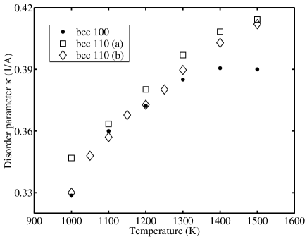
Figure 1: The disorder parameter $\kappa$ for bcc substrates. The results are very similar for both the (110) and (100) substrates at $T\leq 1300K$.

For low temperatures (approximately $T<1300$K) there is no substantial difference in $\kappa$ between all systems, i.e. the amount of disorder exhibited at each interface is the same. However, for higher temperatures ($T>1300$K) the (100) and (110) systems deviate substantially, and the (100) system is seen to preserve more order at higher temperatures than the (110) system.

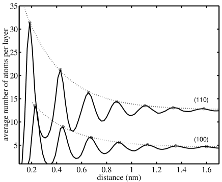
Figure 2: Layering in the liquid for bcc (100) and bcc (110) substrates at 1000K. The graph shows the average number of atoms per layer as a function of distance (in the z direction) in nm from the substrate. Only the part of the liquid adjacent to the solid is shown, and the average number of atoms in each layer is plotted as a function of the distance from the solid substrate.

The proximity of $\kappa$ at low temperatures can be further demonstrated from the comparison of the density profiles of the two systems in Figure 2. The average number of atoms in each layer is plotted as a function of the distance of the layer from the solid substrate at a temperature of $T=1000$K. The peaks corresponding to the solid phase are not shown. Note that the y-axis is the average number of atoms found in each layer and not the density. The layer magnitude, or average number of atoms in each layer, decays gradually to a constant value. When this value is normalized by the volume of each layer, it will be equal to the density of the liquid, which is the same for all systems. The dashed lines are an actual fit to Equation 1. Despite the difference in the magnitude and the distance from the substrate, both profiles are very similar, with the same number of density peaks, and a very similar envelope (dashed lines). Hence it is not surprising that $\kappa$ is very close for both systems.

Since both the in-plane structures and the d-spacings of the bcc (110) and bcc (100) substrates are different, we would expect that some of this difference be reflected in the structure of the liquid at the interface. However we obtain very similar results for both $\kappa$, and for the density profiles.

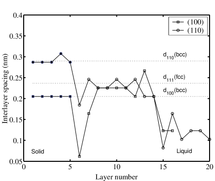
Figure 3: The d-spacing for bcc (100) and bcc (110) substrates; in both cases the interlayer spacing inside the liquid is compatible with the periodicity of (111) planes in an fcc metal.

We next examine the interlayer spacing for both systems, as shown in Figure 3. The closed symbols indicate the d-spacing found in the ideal structure (the small solid peak in the case of the (110) system is due to a small shift in the slicing). In both systems the interlayer distance of the quasi-liquid is uncorrelated with the d-spacing of the substrate. This suggests that in both cases the in-plane structure in the liquid is not similar to that of the substrate. Moreover, apart from first layer in each system, the interlayer spacing in both cases is seen to fluctuate around a value which is close to the d-spacing of a (111) family of planes in an ideal fcc material. The drop in the d-spacing of the first layer for the (110) system is mainly an artifact of the slicing scheme as noted earlier. The large drop in the d-spacing of the first layer for the (100) system is however, related to a physical phenomenon that is explained below.

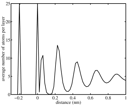
Figure 4: The profile of the bcc (100) system showing an extra peak very near to the solid peak, which is due to the adsorbed liquid layer.

Figure 4 shows the density layering in the (100) system, with a closer look at what happens near the rigid substrate. The first two peaks shown correspond to the solid substrate. In addition to the layers well inside the liquid, there is an additional peak in the density profile, very close to last peak of the substrate. This peak leads to the substantially low inter-layer spacing for the first peak in Figure 3. A better understanding of the source of this peak is achieved by looking at the actual structure of the interface, as shown in Figure 5. The left panel is a side view, looking down from the [010] direction, of a part of the interface showing the last two solid layers, labeled (a), and (b), and the two liquid layers adjacent to the substrate, labeled (c) and (d). The right panel is a top view, looking down from the [100] direction. The size of the atoms drawn in the right view was changed to make it easier to discern the different layers. Layer (a) is drawn with larger black spheres, followed by smaller dark spheres for layer (b). It is clear that the extra peak in Figure 4 is due to the layer (c) (dark gray atoms in Figure 5) formed by the liquid atoms that penetrate - or adsorb - into the terminating plane of the rigid substrate. These atoms fall into the face-centered positions of the bcc (100) plane, immediately above the positions of the atoms in layer (a), in accordance with the fcc interaction potential of the liquid. In this way, the terminating plane of the bcc (100) material transforms, via the adsorption of the liquid, into an fcc (100) plane. Note that half of the atoms in this plane are rigid and the other half slightly displaced above the ideal positions of the face-center atoms. Hence we expect that the structure of the liquid at the bcc (100) substrate will be very similar to that found at an actual fcc (100) substrate.

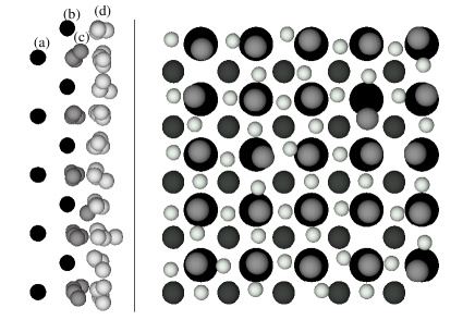
Figure 5: The interface region at a bcc (100) substrate at $T=1000K$. The left panel is a side view and the right panel is a top view. The darkest atoms represent the solid, medium and light gray, the liquid. On the right, different sizes indicate layer position: layer (a) is represented by large spheres, layers (b) and (c) by normal size, and layer (c) by a smaller size. Liquid atoms (dark gray) in layer (c) are adsorbed into the solid, they lie in the face-centered sites on the bcc (100) plane, but positioned slightly above the (100) plane as seen from the left panel.

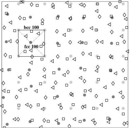
Figure 6: Stacking of layers in the bcc (100) system at $T=1000K$. Light gray circles represent atoms in the terminating bcc (100) plane, dark gray circles the adsorbed layer, diamonds, squares, and triangles represent the first three layers in the liquid. The square connects four atoms of the bcc (100) plane, and the dark circle in the middle indicates the additional site of the fcc (100) plane, occupied by an adsorbed atom.

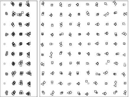
Figure 7: Stacking of layers in the bcc (100) system at $T=600K$. Symbols are the same as for Figure 6, but the metallic region has now solidified, forming a bcc (100)/fcc (100) interface.

.

In the discussion so far, and in what follows, we assume that the adsorbed liquid layer is part of the terminating plane of the solid, so that when calculating $\kappa$ we have excluded this peak from the density envelope (see Figure 2).

We now turn our attention to the first liquid layer, labelled (d) and shown in light gray in Figure 5. The atoms of this layer fall into sites directly above holes in the terminating substrate. There exists a large amount of order in this layer, as can easily be seen from the right panel of Figure 5. The location of the second and third liquid layers is shown in Figure 6. The atoms in the second layer fall into well defined sites, above the holes in the first layer, and above atoms in layer (b). In order to see more clearly the actual stacking of the planes in the liquid phase, we cool down the sample and let the atoms settle into their equilibrium structures. Figure 7 shows a snapshot of a sample solidified at $T=600$K. The stacking of the planes shown and the position of the atoms indicates the formation of (100) fcc planes.

On the other hand, the in-plane ordering in the BCC (110) system is much less pronounced as can be seen from Figure 8, which shows the structure near the interface at 1000K, the last two solid planes (darkest atoms), and the first two liquid layers (medium and light gray). The left panel is a side view, looking down from a $(0\bar{1}1)$ direction, and the right panel is a top view, looking down from the (110) direction. It is hard to quantify the amount of order inside the layers from just looking at the configuration, although one can clearly see that some order exists, at least short range order, which resembles a bcc (110) plane. The ordering inside the planes does not improve much by cooling down the sample.

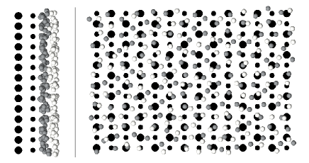
Figure 8: The interface region at a bcc (110) substrate at $T=1000K$. The left panel is a side view and the right panel is a top view. The darkest atoms represent the solid, medium and light gray, the liquid. Different sizes indicate layer position as can be seen from the left panel. In contrast to the (100) system, there is no adsorption of the liquid to the solid substrate. Partial ordering exists in the liquid layers in the manner of a (110) system, however many defects are present in the system (see text).

To summarize, comparing the ordering for both systems, there seems to be a qualitative difference between ordering normal to the interface, and ordering inside the planes. Normal to the plane of the interface the order in both systems is identical, both in terms of $\kappa$ and of the d-spacing. However, the in-plane structure is strongly correlated with the underlying substrate, which is very different in both cases. In addition, the bcc (100) substrate is strongly affected by the adsorption of additional aluminium atoms from the liquid phase, while this effect does not occur with the bcc (110) substrate. Effectively, we are actually comparing an interface with a fcc (100) substrate and an interface with a bcc (110) substrate.

Systems with an fcc substrate were investigated in a previous report [3], where fcc substrates with three different terminating planes were simulated: (111), (100), and (110). The disorder parameter $\kappa$ for the (111) and (100) fcc substrates varied faster with temperature than the one obtained here for the bcc substrates. At low temperature, $\kappa$ for the fcc substrates was smaller, and at high temperature larger, than $\kappa$ for the bcc substrates. This difference is particularly surprising in view of the similarity of the fcc (100) and bcc (100) interfaces, which results from the absorbed layer. At present we have no simple explanation of the difference. The disorder parameter, $\kappa$ for the fcc (110) substrate was much larger than for the other fcc and bcc substrates, and increased almost linearly with temperature. The interlayer spacing in the liquid phase for the fcc (111) and (100) was very similar to the d-spacing in the bcc systems, that is in all cases it was very close to the d-spacing of an fcc solid ($d_{111}=2.367$Å). The interlayer spacing in the fcc (110) system was equal to the d-spacing of the underlying substrate. In conclusion, for the fcc system, the interlayer spacing in the liquid is comparable to the interlayer spacing inside the fcc substrate.

For the fcc systems, it was also observed that the density changes gradually to that of the bulk liquid over the interface region. Inside the interface region there exists a strict correlation between the interlayer spacing and the in-plane density in the form of the in-plane density $\zeta$ normalized by the interlayer spacing $d$:

$$\rho=\zeta/d$$ (2)

where $\rho$ is the bulk density in each layer. For a perfect lattice this relation is exact, i.e. $\rho$ is the bulk density of the whole sample. At the interface region $\rho$ gradually decays across the interface to the density in the bulk liquid.

For a system with an fcc substrate the difference in density accross the interface is not large; the density of the fcc substrate being $\rho_{fcc}=0.058$ atoms/ų (with the lattice paramter of $4.1$Å), while that of liquid aluminium within our temperature range is about $\rho_{Al}=0.052$ atoms/ų. Hence there is no substantial change in the density of the liquid layers, and consequently there was no major change in the interlayer spacing (see Equation 2).

In contrast to the fcc case, the bcc systems are much less dense than both solid and liquid aluminium (the density of the bcc substrates is $\rho_{bcc}=0.029$ atoms/ų). The liquid near the interface must then accomodate for this change in the density across the interface.

When the liquid metal is adjacent to the solid, there will be an interplay, or competition between the solid and the liquid; the liquid wants to equilibrate to it’s natural density, while the bcc substrates tend to impose their symmetry on the liquid. In the case of the bcc (100) substrates, the liquid dominates. The terminating plane of the bcc (100) is transformed by the “adsorption of the liquid” into an fcc (100) plane, which is much denser than bcc (100). Indeed this interface behaves similar to one with a true fcc (100) substrate [3].

In the case of the bcc (110) system the situation is more complicated. Again, the liquid tends to order, but the bcc (110) imposes its in-plane structure onto the liquid. The system will reach a certain equilibrium between these two effects. This is exactly what happens in Figure 8, where part of the plane is ordered in a (110) symmetry, and the other is not, while the density in the liquid layers is typical for liquid aluminium. Table 1 lists the average in-plane density and the interlayer separation for the bcc (110) system at a temperature of $T=1000$K. The first layer is from the perfect lattice, and the rest is the liquid interlayer density. The values of the perfect in-plane densities for the various surfaces considered here are also listed for comparison. We note that the density of the first layer adjacent to the bcc (110) plane jumps to a value very close to the density of an ideal fcc (111) or (100) plane. When this density is normalized by the interlayer separation, it is very close to the bulk liquid density. This causes the change in the d-spacing for the (110) system from the bcc (110) value of $d_{110}=2.8991$Å, to a value close to an fcc (111).

bcc (110)			ideal lattices
layer	$d$	$\zeta$ atoms/Å2	plane	$\zeta$ atoms/Å2
1.	2.8700	0.0841	bcc (100)	0.0594
3.	2.4600	0.1219	bcc (110)	0.0841
4.	2.2550	0.1202	fcc (111)	0.1374
5.	2.2550	0.1150	fcc (100)	0.1190
6.	2.2550	0.1056	fcc (110)	0.0841

Table 1: The width and density of the liquid layers at the interface with a bcc (110) substrate (left), compared to the planar densities for different ideal planes (right). All models are with a lattice parameter of $a=4.1$Å.

4 Summary and Conclusions

We have simulated liquid Al in contact with bcc substrates, and compared the results with similar systems having fcc substrates. We study the oscillations in the density perpendicular to the interface and their decay profile as a function of temperature. The envelope of the density fluctuation is well described by an exponential, $a\exp{(-\kappa z)}+b$, where $\kappa$ is a measure of the disorder at the liquid. We find that the ordering normal to the plane of the interface is similar for both systems, despite a very different structure of the underlying substrates, and that it is dominated by the properties of the liquid material. On the other hand, the effect of the in-plane structure of the substrate is rather pronounced. For the (100) system, the liquid is much more ordered than for the (110) system. This is because additional atoms from the liquid phase adsorb into face centered sites in the bcc (100) surface, forming a structure resembling solid fcc (100). Work is in progress to understand the relatively small temperature dependence of the disorder parameter $\kappa$ on bcc compared to fcc substrates.

Acknowledgements A.H. was supported by the Israeli Ministry of Science. This research was partially supported by the German-Israel Science Foundation under grant I-653-181.14/1999, and by the Binational Science Foundation (Israel-USA, BSF Grants 1998102 and 1999200).

References

- [1] W. J. Huisman, J. F. Peters, M. J. Zwanenburg, S. A. de Vries, T. E. Derry, D. Aberanathy, and J. F. Van der Veen, Nature, 390, 379, (1997)
- [2] H. Reichert, O. Klein, H. Dosch, M. Denk, V. Honklmaki, T. Lippmann, G. Reiter, Nature, 408, 839, (2000)
- [3] Adham Hashibon, Joan Adler, Michael W. Finnis, and Wayne D. Kaplan, Submitted to Computational Material Science, September 2001.
- [4] J.M. Howe, Phil. Mag. A, 74, 761 (1996), and references therein.
- [5] F. Ercolessi, and J. B. Adams, Euro. Phys. Lett., 26, 583 (1994)
- [6] D. Frenkel, and B. Smit, “Understanding Molecular Simulation, from Algorithms to Applications”, Academic Press 1996.
- [7] M.P. Allen, and D.J. Tildesley, Computer Simulation of Liquids, Oxford University Press, 1987.
- [8] F. Ercolessi, E. Tosatti, and M. Parrinello, Phys. Rev. Lett. 57, 719 (1986); F. Ercolessi, M. Parrinello, and E. Tosatti, Phil. Mag. A 58, 213 (1988).
- [9] U. Hansen, P. Vogl, and V. Fiorentini, Phys. Rev. B., 60, 5055, (1999)
- [10] O. Tomagnini, F. Ercolessi, S. Iarlori, F.D. Di Tolla, and E. Tosatti, Phys. Rev. Lett., 76, 1118, (1996)
- [11] P. Tarazona and L. Vicente, Mol. Phys., 56, 557, (1985)