From Linear to Nonlinear Response in Spin Glasses:
Importance of Mean-Field-Theory Predictions

Abstract

Deviations from spin-glass linear response in a single crystal Cu:Mn 1.5 at % are studied for a wide range of changes in magnetic field, $\Delta H$. Three quantities, the difference $TRM-(MFC-ZFC)$, the effective waiting time, $t_{w}^{e\!f\!f}$, and the difference $TRM(t_{w})-TRM(t_{w}=0)$ are examined in our analysis. Three regimes of spin-glass behavior are observed as $\Delta H$ increases. Lines in the $(T,\Delta H)$ plane, corresponding to “weak” and “strong” violations of linear response under a change in magnetic field, are shown to have the same functional form as the de Almeida-Thouless critical line. Our results demonstrate the existence of a fundamental link between static and dynamic properties of spin glasses, predicted by the mean-field theory of aging phenomena.

I Introduction

The properties of spin glasses in a magnetic field have been the subject of considerable attention. It is widely recognized that the Parisi replica-symmetry breaking ansatz mez87 provides an essentially correct mean-field solution for the infinite-range Sherrington-Kirkpatrick model. she75 The spin-glass phase in this model is separated from the paramagnetic phase in the $(T,H)$ plane by the de Almeida-Thouless (AT) critical line. alm78 The situation is less clear in the case of finite-dimensional short-range models. Rigorous theoretical results show viability of the mean-field approach for the description of these systems, mar00 but progress is impeded by significant analytical difficulties. Numerical studies have repeatedly suggested the existence of an AT-type critical line at $d=3$ and higher dimensions. car90 ; zul98 However, magnetic field effects present a difficult challenge for computer simulations. Finite size, and difficulties in equilibrating large samples, do not yet allow a clear distinction between the mean-field picture and the droplet scenario. krz01 Because of this, the existence of the spin-glass phase transition in a magnetic field is considered a most relevant open problem.zul98

The experimental evidence for an AT-type critical behavior appears ambiguous. Many real spin glasses have mean-field-like phase diagrams, ken91 with an onset of strong $MFC-ZFC$ irreversibility along a certain line. This irreversibility is usually interpreted as a sign of replica-symmetry breaking. However, real spin glasses are always out of equilibrium, and the measured AT lines are time dependent. Therefore, it appears impossible to obtain information about the equilibrium phase diagram directly from experiments. We show in this paper, however, that the study of magnetic field effects on the nonequilibrium dynamics of spin glasses can shed light on the magnetic properties of the equilibrium spin-glass state.

Our motivation for this work is twofold. First, effects of magnetic field are understood fairly well within the mean-field theory, where they are derived from first principles. The minimum possible overlap, $q_{min}(H)$, of two states in the presence of a magnetic magnetic field, $H$, plays an important role in this approach. Yet, as usually happens in spin-glass physics, the theoretical predictions cannot be easily related to experimentally observable phenomena. Even those models of spin-glass dynamics that are based on the mean-field-like hierarchical picture of phase space tend to treat magnetic field effects phenomenologically in terms of the Zeeman energy. In this paper, we show that experimental results on the magnetic field dependence of spin-glass dynamics are consistent with the mean-field description.

The second reason for this work is practical. Spin-glass relaxation properties are usually studied under a change in magnetic field. It is often believed that the subsequent response is linear in magnetic field “for reasonably small field values (say $<10~{}G$)”. kop88 We show in this paper that the very definition of what one means by “reasonably small” fields is impossible without knowledge of the spin-glass phase diagram. This knowledge becomes vital when results for different temperatures or different samples are compared.

The paper is organized as follows. The next Section describes a theoretical picture underlying our analysis. Sec. III.A presents results of magnetization measurements. Sec. III.B is devoted to experimental results for the effective waiting time. In Sec. III.C, the waiting-time dependence of the measured quantities is discussed in detail. Sec. IV summarizes our conclusions.

II Theoretical background

II.1 Mean-field dynamics

The main obstacle to an experimental test of mean-field-theory predictions is the problem of relating experimentally accessible spin-glass dynamics to the static equilibrium properties of the spin-glass state, described by the Parisi solution. Phenomenological phase-space models have provided important insights into possible physical mechanisms for spin-glass relaxation.led91 ; bou92 A recent theoretical breakthrough has been achieved within the mean-field theory of aging phenomena, proposed by Cugliandolo et al. cug93 ; fra95 ; mar98 ; fra98 Because these theoretical developments have profound significance for the interpretation of our experimental results, we shall briefly review them here.

The well-known fluctuation-dissipation theorem (FDT) kub66 establishes a link between the linear response of a system to an external perturbation, and the fluctuation properties of the system in thermal equilibrium. The response of a spin system at time $t$ to an instantaneous field at time $t^{\prime}$, $R(t,t^{\prime})$, and the spin autocorrelation function, $C(t,t^{\prime})$, are defined as follows:

$$R(t,t^{\prime})=(1/N)\sum_{i=1}^{N}\delta\langle S_{i}(t)\rangle/\delta h(t^{\prime})~{}~{};$$ (1)

$$C(t,t^{\prime})=(1/N)\sum_{i=1}^{N}\langle S_{i}(t)S_{i}(t^{\prime})\rangle~{}~{}.$$ (2)

In thermodynamic equilibrium, both functions are time-translation invariant, and related by the fluctuation-dissipation theorem ($\beta=1/k_{B}T$):

$$R_{eq}(t-t^{\prime})=\beta\partial C_{eq}(t-t^{\prime})/\partial t^{\prime}~{}~{}.$$ (3)

The violation of this theorem in a general off-equilibrium situation is described by the function $X(t,t^{\prime})\leq 1$: cug93 ; fra95 ; mar98

$$R(t,t^{\prime})=\beta X(t,t^{\prime})\partial C(t,t^{\prime})/\partial t^{\prime}~{}~{}.$$ (4)

Violation of the fluctuation-dissipation theorem is associated with a deviation from linear response. A second-order nonlinearity does not appear because the magnetization changes sign when the field is reversed. It has been shown lev89 that the presence of a third-order nonlinear response turns the fluctuation-dissipation theorem into a fluctuation-dissipation inequality. This is consistent with the fact that $X(t,t^{\prime})$ in Eq. (4) is generally less than unity.

When these formulas are applied to spin-glass dynamics, the relevant times are $t=t_{w}+\tau$ and $t^{\prime}=t_{w}$, where $t_{w}$ and $\tau$ are the waiting time and observation time after the waiting time, respectively. The dynamical quantities $C$ and $X$ can be related to their equilibrium counterparts if both $t_{w}$ and $\tau$ are sent to infinity. However, time-translational invariance does not hold off equilibrium, and the limiting values depend on how the limits are taken. One can write for the correlation function, bou97 ; cug99

$$\lim_{\tau\rightarrow\infty}\lim_{t_{w}\rightarrow\infty}C(t_{w}+\tau,t_{w})=q_{EA}~{}~{},$$ (5)

and

$$\lim_{\tau\rightarrow\infty}C(t_{w}+\tau,t_{w})=q_{min}~{}~{}.$$ (6)

Eq. (5) is a dynamical definition of the Edwards-Anderson order parameter, $q_{EA}$, as the value of the correlation function at the limit of validity of the fluctuation-dissipation theorem. Eq. (6) expresses the property of weak ergodicity breaking in spin glasses. If the waiting time is finite and the magnetic field is zero (giving $q_{min}=0$), the system is able to escape arbitrarily far from the configuration it had reached at $t=t_{w}$. bou97

The fluctuation-dissipation ratio $X(q)$ is defined as the limit of the function $X(t,t^{\prime})$, taken along a path in the $(t,t^{\prime})$ plane, characterized by a given value $q$ of the correlation function $C(t,t^{\prime})$.fra98 The most important result of the theory is the fact that, under the assumption of stochastic stability,fra98 $X(q)$ is equal to the equilibrium order parameter function $x(q)$:

$$X(q)=\lim_{t,t^{\prime}\rightarrow\infty;~{}C=q}\frac{R(t,t^{\prime})}{\beta\partial C(t,t^{\prime})/\partial t^{\prime}}=x(q)~{}~{}.$$ (7)

The function $x(q)$ is an integral of the Parisi order parameter $P(q)$,mez87 which can be introduced for short-range spin glasses within the standard replica-symmetry breaking formalism. mar00 According to Eq. (7), there is a deep relationship between spin-glass dynamics and the static equilibrium properties of the spin-glass state. It implies that “in any finite-dimensional system, replica-symmetry breaking and aging in the response functions either appear together or do not appear at all”. fra98

We now consider the physical (experimental) significance of these theoretical results. It is well known that there are two main regimes of spin-glass relaxation. In the equilibrium, or stationary regime, observation times $\tau\ll t_{w}$, the fluctuation-dissipation theorem holds and the response function depends only on $\tau$. In the nonequilibrium, or aging regime, observation times $\tau>t_{w}$, the FDT is violated and the relaxation depends on $t_{w}$ for any $\tau$. Both regimes have been observed experimentally oci85 and studied numerically.fra95 ; and92 The transition from one regime to the other is marked by a peak in the relaxation rate, corresponding to strong violation of FDT at $\tau\approx t_{w}$.

These effects can be naturally explained within the mean-field theory of aging phenomena. It has been suggested cug93 that the function $X(t,t^{\prime})$, introduced to describe violations of the FDT in Eq. (4), depends on its time arguments only through the correlation function: $X=X[C(t,t^{\prime})]$. In the equilibrium regime, the correlation function decreases rapidly (on the linear time scale) from 1 to $q_{EA}$, and $X(C)=1$. In the aging regime, the correlation function relaxes slowly from $q_{EA}$ to $q_{min}$, and $X(C)<1$. cug99 ; par98 The transition from one regime to the other is a direct consequence of replica-symmetry breaking at $q<q_{EA}$.

II.2 Chaotic nature of the spin-glass state

Another important issue is the chaotic nature of the spin glass state with respect to magnetic field. It has been demonstrated numerically that a small change in external field leads to a considerable reorganization of a spin configuration.ban81 The Parisi solution suggests that an average equilibrium overlap between two states at different but similar magnetic fields, $(h_{1}-h_{2})^{2}N\gg 1$,mar00 is equal to $q_{min}$, i.e. the minimum possible overlap.par83 Analysis of fluctuations around the Parisi solution, carried out by Kondor,kon89 demonstrates that the correlation overlap function $C_{H}(r)$ for two spins, $i$ and $j$, at a distance $r$, behaves as

$$C_{H}(r)=\overline{\langle S_{i}S_{j}\rangle_{H}\langle S_{i}S_{j}\rangle_{0}}~{}\propto~{}\exp(-r/\xi_{H})~{}.$$ (8)

This means that the projection of the correlation $\langle S_{i}S_{j}\rangle_{H}$ at field $H$ onto the correlation $\langle S_{i}S_{j}\rangle_{0}$ at zero field vanishes beyond the finite characteristic length $\xi_{H}$. Near $T_{g}$ and at low fields, this magnetic correlation length is simply $\xi_{H}=1/q_{min}(H)$. In the mean-field theory, $q_{min}(H)\propto H^{2/3}$, so that $\xi_{H}$ diverges rapidly as the field goes to zero.

The behavior of the correlation function, Eq. (8), is a consequence of replica-symmetry breaking. The low-temperature spin-glass phase has an essentially infinite number of pure equilibrium states. Each of them is characterized by an infinite correlation length. These states have equal free energies per site, except for differences of the order $O(1/N)$. Only a few states with the lowest energies contribute significantly to the partition function. Because of the small energy differences, any small (but finite) amount of energy, added to the system, is enough to reshuffle the Boltzmann weights of the different states and thus completely reorganize the equilibrium spin configuration. Application of a magnetic field is an example of such a perturbation.

The magnetic correlation length, $\xi_{H}$, has the following meaning.rit94 When a magnetic field $H$ is applied to the system, the minimum possible overlap of two states is equal to $q_{min}(H)$. Consequently, all the states having overlaps $q<q_{min}$ are suppressed by the field. Their free energies increase, and they acquire the finite correlation length $\xi_{H}$. The spatial spin correlations, corresponding to these states, survive only within this range. All the other pure states are still characterized by an infinite correlation length. At the AT line, where $q_{min}=q_{EA}$, all the states have a finite correlation length, and the system becomes paramagnetic. Thus, a change in magnetic field has a randomizing effect on the spin-glass state. The ratio $q_{min}/q_{EA}$ is a natural measure of this effect.

The chaotic nature of the spin-glass state is also reflected in the phenomenological droplet model. The magnetic correlation length is determined as an average droplet size for which the Zeeman energy is equal to the energy of the droplet excitation. It is given by the following expression:fis88

$$\xi_{H}\propto H^{-2/(d-2\theta)}~{}.$$ (9)

Even though this result, with $d=3$ and $\theta\approx 0.2$, is similar to the result of the mean-field theory, the physics is quite different. Spin-glass properties in this model are governed by low-energy excitations of the ground state, created by coherent flipping of compact clusters of spins. It is suggested that the magnetic field, $H$, would flip all the droplets with sizes greater than $\xi_{H}$ and thus destroy all spin-glass correlations beyond this length scale. Therefore, at any nonzero field, there is only a paramagnetic state with the finite correlation length $\xi_{H}$.

In both these approaches, the chaotic nature of the spin-glass state with respect to magnetic field leads to departures from linear response as $\Delta H$ increases.

III Experimental results and analysis

The purpose of this paper is the study of violations of the fluctuation-dissipation theorem as a function of magnetic field change $\Delta H$. According to Eq. (7), aging dynamics of the spin-glass state is ultimately determined by static equilibrium properties. Any violation of the FDT contains information about replica-symmetry breaking. Therefore, studies of the gradual deviation from linear response as $\Delta H$ increases can provide insight into the nature of the spin-glass phase diagram. Direct experimental determination of the correlation function, Eq. (2), requires sophisticated measurements of the time dependent magnetic noise spectrum.bou88 Instead, we make use of quantities which can be obtained from magnetic susceptibility measurements. The first quantity of interest is the difference of the values of remanence, measured in TRM and ZFC experiments: $TRM-(MFC-ZFC)$. It has been shown lun86 that, within the linear regime, this quantity is zero, provided that all three magnetizations are measured at the same time after the initial quench. The second quantity of interest is the effective waiting time, $t_{w}^{e\!f\!f}$, defined as the value of the observation time $\tau$ where the relaxation rate $S(\tau)=-\partial TRM(\tau,t_{w},\Delta H)/\partial\log\tau$ has a maximum. It has been argued dju95 that, within the linear response regime, $t_{w}^{e\!f\!f}\approx t_{w}$, so that the peak in $S(\tau)$ is essentially unaffected by a small magnetic field change. The third quantity we study experimentally is the difference $TRM(t_{w})-TRM(t_{w}=0)$. It describes a change in the measured magnetization as a result of the waiting time, and thus allows closer examination of aging phenomena.

All experiments were performed on a single crystal of Cu:Mn 1.5 at %, a typical Heisenberg spin glass with a glass temperature of about $15.2~{}K$. Results of conventional studies of the phase diagram for this sample will be reported elsewhere. A commercial Quantum Design SQUID magnetometer was used for all the measurements.

III.1 Measurements of $TRM$, $MFC$, and $ZFC$

Fig. 1 exhibits the dependence of $TRM$, $MFC-ZFC$, and their difference, on the field change $\Delta H$, measured at $T=12.0~{}K$. All data points were taken at the same short observation time, $\tau\approx 40~{}s$, with zero waiting time, and an effective cooling time of about $600~{}s$. Error bars are smaller than the symbol sizes. The same will apply to all figures without error bars. Fig. 1 shows that three different types of spin-glass behavior can be distinguished for different ranges of magnetic field change, $\Delta H$. For field changes from $\Delta H=0$ to $\Delta H_{1}\approx 120~{}Oe$, the difference $TRM-(MFC-ZFC)$ is zero to within our experimental accuracy. Between $\Delta H_{1}$ and $\Delta H_{2}\approx 420~{}Oe$, there are weak deviations from linear response. At $\Delta H=\Delta H_{2}$, corresponding approximately to the peak in the $MFC-ZFC$ remanence, violation of linear response becomes strong, and the difference $TRM-(MFC-ZFC)$ is a linear function of $\Delta H$ with a large slope.

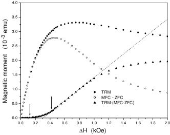
Figure 1: The values of the remanent magnetic moment, measured at $T=12.0~{}K=0.79~{}T_{g}$ and $t_{w}=0$. The magnetic field is changed from $H=\Delta H$ to $H=0$ (TRM experiment) and from $0$ to $\Delta H$ (ZFC experiment). The two arrows indicate the critical field changes, $\Delta H_{1}\approx 120~{}Oe$ and $\Delta H_{2}\approx 420~{}Oe$, for the weak and strong linear response violations, respectively.

The temperature dependences of the critical field changes $\Delta H_{1}$ and $\Delta H_{2}$ are presented in Fig. 2 and Fig. 3. The figures also show the critical AT line, determined for the same sample at the same observation and cooling times, using the onset of strong $MFC-ZFC$ irreversibility as the signature of the spin-glass phase transition. We assume that this dynamical line approximates the equilibrium AT line for infinite waiting time. The difference $MFC-ZFC$ in Fig. 1 is not zero at the AT field of $\approx 1400~{}Oe$ because transverse freezing above the AT line leads to a weak longitudinal irreversibility.gab81

Figure 2: The dynamical AT line $\Delta H_{AT}(T)$, the strong linear response violation line $\Delta H_{2}(T)$, and the weak linear response violation line $\Delta H_{1}(T)$, determined from the linear fits to experimental data, plotted as $\Delta H^{2/3}$ vs. $T$.

Figure 3: The same lines as in Fig. 2, but plotted as $\Delta H(T)$. Note that the two linear response violation lines below the AT line represent a dynamic crossover from one relaxation regime to the other. They are not features of an equilibrium phase diagram.

One sees from Fig. 2 that all three lines in the $(T,\Delta H)$ plane have the same functional form, $T_{g}-T=a\Delta H^{2/3}$, typical of the equilibrium AT critical line alm78 in the SK model. Moreover, the two linear-response violation lines, $\Delta H_{1}(T)$ and $\Delta H_{2}(T)$, determine dynamical transition temperatures which are very close to the actual glass temperature $T_{g}$. It would thus be incorrect to say that the critical AT-type line plays a role at high fields only. Our results demonstrate that this line manifests itself dynamically even at very low fields. A critical field change for a given degree of linear response violation seems to be a constant fraction of the AT field. It means, from a practical point of view, that results obtained at different temperatures can be directly compared only if they have the same $\Delta H/H_{AT}(T)$ ratio.

A comment should be made at this point. It has been argued wen84 that a $T\propto H^{2/3}$ dependence for transition lines is not a unique feature of the mean-field theory. A similar power law could be obtained from purely dynamical considerations without using the concept of the spin-glass phase transition.wen84 A dynamical freezing line, $T_{f}(H,\omega)$, appears in the droplet model as well.fis88 In the present analysis, we do not rely on the existence of the $H^{2/3}$ dependence by itself. Our argument is based on the fact that the experimental AT and linear response violation lines have the same functional form, as illustrated in Fig. 2 and Fig. 3. This result suggests that there is a close relationship between the static and dynamic properties of the spin-glass state, assuming that the measured AT line is related to the equilibrium one.

Of course, measured values of the critical field changes depend on both the waiting time and the observation time. This point is illustrated in Fig. 4 where values of $TRM-(MFC-ZFC)$ are plotted for $t_{w}=0$ and $t_{w}=30~{}min$. As the waiting time becomes larger, $\Delta H_{1}$ increases, while $\Delta H_{2}$ decreases. Thus, longer equilibration times make the system less susceptible to external perturbations, but only up to a certain point. This issue will be discussed further in Sec. III.C.

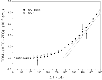
Figure 4: The function $TRM-(MFC-ZFC)$, describing violation of linear response, at $t_{w}=30~{}min$ and $t_{w}=0$. The second and the third arrows from the left indicate, respectively, the larger value of $\Delta H_{1}$ and the lower value of $\Delta H_{2}$ for the longer waiting time.

III.2 Measurements of the effective waiting time

Let us now turn to a discussion of the effective waiting time, $t_{w}^{e\!f\!f}$. Fig. 5 exhibits the dependence of $\log_{10}(t_{w}^{e\!f\!f})$ on the magnetic field change $\Delta H$ for three different waiting times: $t_{w}=30~{}min,~{}5~{}min$, and 0. The temperature is the same as in Fig. 1. One can easily discern three regimes of FDT violation, corresponding to the three regimes of deviation from linear response seen in Fig. 1.

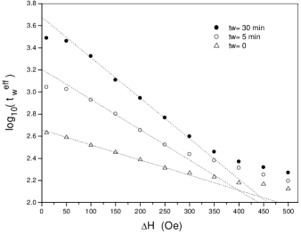
Figure 5: Logarithm of the effective waiting time, $t_{w}^{e\!f\!f}$, as a function of $\Delta H$, measured at $T=12.0~{}K=0.79~{}Tg$ for three waiting times. The dotted lines are linear fits in the interval $100...250~{}Oe$. They are only guides for the eye.

As the magnetic field change, $\Delta H$, increases from zero up to about $100~{}Oe$, the effective waiting time decreases only slightly. This means that FDT holds for observation times less than $t_{w}^{e\!f\!f}\approx t_{w}$. Of course, if the waiting time is short, $t_{w}^{e\!f\!f}$ is determined by the cooling procedure.

In the interval from $100~{}Oe$ to about $400~{}Oe$, the effective waiting time drops sharply, and the field dependence of its logarithm is linear. In this case, nonequilibrium behavior appears much earlier, and the FDT holds only at short times $\tau\ll t_{w}^{e\!f\!f}\ll t_{w}$. This corresponds to the weak deviation from linear response between $\Delta H_{1}$ and $\Delta H_{2}$ in Fig. 1.

When the field change exceeds $400~{}Oe$, the FDT is strongly violated. One can see from Fig. 5 that, in this regime, the curves for long waiting times approach the curve for zero waiting time, and the waiting time dependence almost disappears. This situation corresponds to the strong deviation from linear response at short observation times above $\Delta H_{2}$ in Fig. 1. Therefore, the break from the linear dependence of $\log_{10}(t_{w}^{e\!f\!f})$ on $\Delta H$, observed at large field changes, is directly related to strong nonlinearity in the spin-glass response. The effective waiting time in this case is determined primarily by the zero waiting time results, dependent on the experimental protocol.

The waiting time dependence in Fig. 5 supports the conclusion, drawn from Fig. 4, that an increase in waiting time leads to an expansion of the linear response region to higher values of $\Delta H$. An increase in the observation time $\tau$ has the opposite effect. The field dependence is more pronounced at longer times. This accounts for the fact that the critical field changes, extracted from the effective waiting time experiments (Fig. 5), seem to be lower than those obtained from the short-time magnetization measurements (Fig. 4). Another interesting feature of our results is that the dependence of $\log_{10}(t_{w}^{e\!f\!f})$ on $\Delta H$ for $t_{w}=0$, determined exclusively by the cooling procedure, does not exhibit the low-field plateau seen at longer waiting times. This behavior is analyzed in Sec. III.C.

The temperature dependence of the effective waiting time is exhibited in Fig. 6 and Fig. 7, where $\log_{10}(t_{w}^{e\!f\!f})$ vs. $\Delta H$ data for $t_{w}=30~{}min$ are plotted for four different temperatures. The results for the smallest field change of $10~{}Oe$ are not exactly the same because the effective cooling time increases as the measurement temperature is lowered. It is quite evident from Fig. 7, however, that the four curves scale rather well together if plotted vs. $\Delta H/\Delta H_{2}$. This means that the critical AT line sets a characteristic magnetic field scale at any temperature below $T_{g}$, and that it plays an important role for all aspects of spin-glass dynamics.

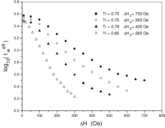
Figure 6: Logarithm of the effective waiting time, $t_{w}^{e\!f\!f}$, measured as a function of $\Delta H$ for $t_{w}=30~{}min$ at four temperatures: $Tr=T/T_{g}=0.70,~{}0.75,~{}0.79$ and $0.85$. Note the similarity in shape and pronounced difference in the magnetic field scales.

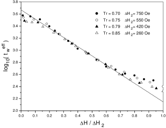
Figure 7: The experimental results of Fig. 6, plotted vs. $\Delta H/\Delta H_{2}$. The critical field change $\Delta H_{2}$, corresponding to strong violation of linear response, is proportional to the AT field, $H_{AT}(T)$. The straight line is a guide for the eye.

III.3 Waiting time dependence of $\Delta H_{1}$ and $\Delta H_{2}$

The waiting time dependences of the characteristic field changes, corresponding to the weak and strong linear response violations, deserve special attention. Our experimental results, exhibited in Fig. 4 and Fig. 5, suggest that $\Delta H_{1}$ increases with $t_{w}$, while $\Delta H_{2}$ diminishes.

In order to check this conclusion, we have measured the field dependence of the thermoremanent magnetization, $TRM(\tau,t_{w},\Delta H)$, for three different waiting times: $t_{w}=30~{}min,~{}5~{}min$, and 0. The measurement temperature is $T=12.0~{}K$, and the observation time after the field change is $\tau=40~{}s$. For convenience, we shall refer to the zero-waiting-time dependence as $ZTRM(\tau,\Delta H)$. This nonequilibrium relaxation function is determined by the cooling process and not by the waiting time. The results are exhibited in Fig. 8. One can see that the maxima in the TRM curves shift towards lower fields as the waiting time increases. To examine evolution of the measured magnetization curves due to aging phenomena, we consider the differences $TRM-ZTRM$, where both $TRM$ and $ZTRM$ are measured at the same observation time. Fig. 8 suggests that the maxima in $TRM-ZTRM$ correspond to higher fields at longer waiting times.

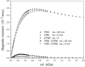
Figure 8: Comparison of $TRM(\Delta H)$ curves measured at $T=12.0~{}K=0.79~{}T_{g}$ for different waiting times. The curve for $t_{w}=0$ is referred to as $ZTRM$. As $t_{w}$ increases, the peak in $TRM$ shifts to the left, while the peak in $TRM-ZTRM$ moves to the right.

Fig. 9 exhibits the logarithm of the ratio $(TRM-ZTRM)/\Delta H$. Two different types of behavior can be clearly distinguished. The ratio increases as long as the field change is less than about $120~{}Oe$, and decreases at higher $\Delta H$. The field dependence of its logarithm can be approximated by straight lines in both regimes. The results in Fig. 9 can be understood if we compare them with the data in Fig. 5. At low field changes, the effective waiting time for $ZTRM$ decreases more steeply with increasing $\Delta H$ than the effective waiting time for $TRM$, which has a plateau in this region. The decay of the $ZTRM$ becomes faster in time, and the ratio $(TRM-ZTRM)/\Delta H$, measured at fixed observation time, increases with $\Delta H$. At higher magnetic field changes the drop in the effective waiting time for the $TRM$ is greater than for the $ZTRM$. As a result, the ratio $(TRM-ZTRM)/\Delta H$ decreases. According to Fig. 9, the transition from one regime to the other occurs at a higher magnetic field change for a longer waiting time. This observation supports our conclusion that the plateau in the field dependence of the effective waiting time broadens as the system equilibrates.

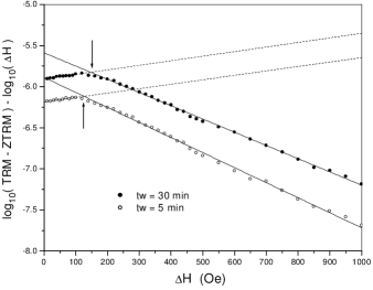
Figure 9: Logarithm of the normalized increase in the thermoremanent magnetization, $(TRM-ZTRM)/\Delta H$, as a function of $\Delta H$ at a constant observation time $\tau=40~{}s$. The dashed lines are linear fits in the interval $0...100~{}Oe$. The solid lines are linear fits in the interval $200...1000~{}Oe$. The arrows indicate points where nonlinearity appears.

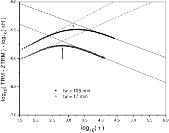
Figure 10: Logarithm of the normalized increase in the thermoremanent magnetization, $(TRM-ZTRM)/\Delta H$, as a function of $\log(\tau)$ at a constant field change $\Delta H=10~{}Oe$. The straight lines are guides for the eye. The arrows indicate transitional points.

Fig. 10 provides further insight into the nature of this effect. It displays the same quantity, the logarithm of $(TRM-ZTRM)/\Delta H$, as a function of time at constant $\Delta H=10~{}Oe$. The experimental protocol is the same as before, except for the different waiting times. One can see a deep similarity between the results in Fig. 9 and Fig. 10. The waiting time dependence exhibited in Fig. 10 is readily understandable: the system stays longer in the quasiequilibrium regime for longer $t_{w}$, so the maximum in $TRM-ZTRM$ shifts towards longer observation times. Comparison with Fig. 9 suggests that the same is true for the field dependence: the system in the quasiequilibrium regime can sustain a stronger perturbation for a longer waiting time.

This similarity between the effects of the observation time and of the field change on the spin-glass state is a natural consequence of replica-symmetry breaking. The weak ergodicity breaking scenario, mentioned in Sec. II.A, suggests that, as the observation time increases, the system can evolve very far from the state at time $t_{w}$, with the minimum correlation set by $q_{min}$. This results from the fact that the average relaxation time is infinite because of the exponential distribution of free energies of different states. Chaotic nature of the spin-glass state with respect to magnetic field, discussed in Sec. II.B, forces the new equilibrium configuration after a field change to have the minimum overlap $q_{min}$ with the old configuration. This phenomenon is also related to existence of an essentially infinite number of states with very similar free energies. Thus, both an increasing observation time and an increasing field change make the spin-glass state less correlated with the state at time $t_{w}$.

It is of interest to examine the waiting time dependences of $\Delta H_{1}$ and $\Delta H_{2}$ for the two “competing” descriptions of spin-glass dynamics: the droplet model and the phase-space picture.

In the droplet model,fis88 if $R(t_{w})$ is an average droplet size, and $L_{\tau}$ is an observation length scale, two limiting cases can be distinguished. For $R(t_{w})\ll\xi_{H}$, the FDT is violated when $L_{\tau}\sim R(t_{w})$, and the field does not play a significant role. For $\xi_{H}\ll R(t_{w})$, the FDT is violated as soon as $L_{\tau}\sim\xi_{H}$, and the waiting time is relatively unimportant. These regimes correspond approximately to experimental regimes with $\Delta H<\Delta H_{1}$ and $\Delta H>\Delta H_{2}$, as discussed above. There is also an intermediate regime with $R(t_{w})\sim\xi_{H}$. This regime is very interesting physically, because violation of the FDT depends on interplay among all three length scales: $L_{\tau}\sim R(t_{w})\sim\xi_{H}$. Unfortunately, no predictions for this regime are given within the droplet model.fis88 It has been arguedkop88 that, if the crossover between linear and nonlinear regimes is defined by a condition $R(t_{w})=\xi_{H}$, the field change, needed to provoke nonlinear relaxation, should decrease with increasing $t_{w}$. This argument can explain the waiting time dependence of $\Delta H_{2}$. However, it fails in the case of $\Delta H_{1}$, which increases with $t_{w}$. Therefore, the experimentally observed waiting time dependence of $\Delta H_{1}$ appears rather counterintuitive within the droplet scenario.

The phase-space picture of spin-glass dynamics does provide a consistent explanation for these phenomena. In this approach, evolution of a system in the phase space can be viewed as a series of transitions among traps, separated by free-energy barriers. bou92 As the system equilibrates, it encounters traps with higher barriers, and these traps increasingly resemble the pure states, contributing to equilibrium.cug93 The quasiequilibrium relaxation regime at short observation times corresponds to evolution within each trap, and the subsequent nonequilibrium behavior is related to evolution from trap to trap. As the waiting time, $t_{w}$, increases, the system has to overcome a higher effective barrier to leave a trap. This takes a longer time, or (if the observation time is fixed) a larger field change. Therefore, the characteristic field change for the weak linear response violation, $\Delta H_{1}$, increases with $t_{w}$. However, after overcoming a higher barrier, the system can explore a broader free-energy landscape due to hierarchical structure of the phase space. It takes less time or a smaller field change to produce a state very different from the one at $t_{w}$. The nonequilibrium behavior is thus more affected by external perturbations for longer waiting times. Therefore, the characteristic field change for the strong linear response violation, $\Delta H_{2}$, decreases with $t_{w}$.

The transition from the quasiequilibrium to the nonequilibrium regime is better defined after longer waiting times, both as a function of the observation time and as a function of the field change. This conclusion agrees with results of numerical simulations, which show the same effect when susceptibility is studied as a function of correlation.fra95

IV Summary

The usual method for studying the spin-glass phase diagram is the observation of the $MFC-ZFC$ irreversibility as a function of temperature at a fixed magnetic field, $H=\Delta H$. A different approach is employed in the present paper. The temperature is kept constant and “ irreversibility of the irreversibility”, $TRM-(MFC-ZFC)$, is measured as a function of magnetic field change $\Delta H$. Increasing $\Delta H$ leads to a gradual deviation from linear response, and, equivalently, to a violation of the fluctuation-dissipation theorem. This violation, according to the mean-field theory of aging phenomena, is directly related to replica-symmetry breaking. Our experiments show that both methods give the same functional form for the critical lines, suggesting a mean-field-like phase diagram. This conclusion is further supported by measurements of the effective waiting time, $t_{w}^{e\!f\!f}$. The study of waiting time effects on the linear response violation suggests the validity of the phase-space picture for spin-glass dynamics. Our results demonstrate the existence of a fundamental link between static and dynamic properties of spin glasses, predicted by the mean-field theory of aging phenomena.

We would like to thank Professor J. A. Mydosh for providing us with the Cu:Mn single crystal sample, prepared in Kamerlingh Onnes Laboratory (Leiden, The Netherlands). We are also grateful to Dr. G. G. Kenning for numerous interesting discussions and to Dr. J. Hammann and Dr. E. Vincent from CEA Saclay (France) for help and advice.

References

- (1) M. Mezard, G. Parisi, and M. A. Virasoro, Spin Glass Theory and Beyond (World Scientific, Singapore, 1987).
- (2) D. Sherrington and S. Kirkpatrick, Phys. Rev. Lett. 35, 1792 (1975).
- (3) J. R. L. de Almeida and D. J. Thouless, J. Phys. A 11, 983 (1978).
- (4) E. Marinari, G. Parisi, F. Ricci-Tersenghi, J. J. Ruiz-Lorenzo, and F. Zuliani, J. Stat. Phys. 98, 973 (2000).
- (5) S. Caracciolo, G. Parisi, S. Patarnello, and N. Sourlas, Europhys. Lett. 11, 783 (1990); E. R. Grannan and R. E. Hetzel, Phys. Rev. Lett. 67, 907 (1991); J. C. Ciria, G. Parisi, F. Ritort, and J. J. Ruiz-Lorenzo, J. Phys. I (France) 3, 2207 (1993).
- (6) E. Marinari, G. Parisi, and F. Zuliani, J. Phys. A 31, 1181 (1998).
- (7) F. Krzakala, J. Houdayer, E. Marinari, O. C. Martin, and G. Parisi, cond-mat/0107366.
- (8) G. G. Kenning, D. Chu, and R. Orbach, Phys. Rev. Lett. 66, 2923 (1991); F. Lefloch, J. Hammann, M. Ocio, and E. Vincent, Physica B 203, 63 (1994) and references therein.
- (9) G. J. M. Koper and H. J. Hilhorst, J. Phys. (France) 49, 429 (1988).
- (10) M. Lederman, R. Orbach, J. Hammann, M. Ocio, and E. Vincent, Phys. Rev. B 44, 7403 (1991); J. Hammann, M. Lederman, M. Ocio, R. Orbach, and E. Vincent, Physica A 185, 278 (1992); Y. G. Joh, R. Orbach, and J. Hammann, Phys. Rev. Lett. 77, 4648 (1996).
- (11) J.-P. Bouchaud, J. Phys. I (France) 2, 1705 (1992); J.-P. Bouchaud and D. S. Dean, J. Phys. I (France) 5, 265 (1995); E. Vincent, J.-P. Bouchaud, D. S. Dean, and J. Hammann, Phys. Rev. B 52, 1050 (1995).
- (12) L. F. Cugliandolo and J. Kurchan, Phys. Rev. Lett. 71, 173 (1993); J. Phys. A 27, 5749 (1994); Phil. Mag. B 71, 501 (1995).
- (13) S. Franz and H. Rieger, J. Stat. Phys. 79,749 (1995).
- (14) E. Marinari, G. Parisi, F. Ricci-Tersenghi, and J. J. Ruiz-Lorenzo, J. Phys. A 31, 2611 (1998).
- (15) S. Franz, M. Mezard, G. Parisi, and L. Peliti, Phys. Rev. Lett. 81, 1758 (1998); J. Stat. Phys. 97, 459 (1999).
- (16) R. Kubo, Rept. Progr. Phys. 29, 255 (1966).
- (17) L. P. Levy and A. T. Ogielski, J. Math. Phys. 30, 683 (1989).
- (18) J.-P. Bouchaud, L. F. Cugliandolo, J. Kurchan, and M. Mezard in Spin Glasses and random fields ed. by A. P. Young (World Scientific, Singapore, 1997).
- (19) M. Ocio, H. Bouchiat, and P. Monod, J. Phys. Lett. (France) 46, L647 (1985); L. Lundgren, P. Nordblad, P. Svedlindh, and O. Beckman, J. Appl. Phys. 57, 3371 (1985).
- (20) J. O. Andersson, J. Mattsson, and P. Svedlindh, Phys. Rev. B 46, 8297 (1992).
- (21) L. F. Cugliandolo, D. R. Grempel, J. Kurchan, and E. Vincent, Europhys. Lett. 48, 699 (1999).
- (22) G. Parisi, Nuovo Cimento D 20, 1221 (1998).
- (23) F. T. Bantilan and R. G. Palmer, J. Phys. F 11, 261 (1981).
- (24) G. Parisi, Phys. Rev. Lett. 50, 1946 (1983); Physica A 124, 523 (1984).
- (25) I. Kondor, J. Phys. A 22, L163 (1989).
- (26) F. Ritort, Phys. Rev. B 50, 6844 (1994); Phil. Mag. B 71, 515 (1995).
- (27) D. S. Fisher and D. A. Huse, Phys. Rev. B 38, 373 (1988); 38, 386 (1988).
- (28) H. Bouchiat and M. Ocio, Comments Cond. Matt. Phys. 14, 163 (1988).
- (29) L. Lundgren, P. Nordblad, and L. Sandlund, Europhys. Lett. 1, 529 (1986).
- (30) C. Djurberg, J. Mattsson, and P. Nordblad, Europhys. Lett. 29, 163 (1995).
- (31) M. Gabay and G. Toulouse, Phys. Rev. Lett. 47, 201 (1981); D. M. Cragg, D. Sherrington, and M. Gabay, Phys. Rev. Lett. 49, 158 (1982).
- (32) L. E. Wenger and J. A. Mydosh, Phys. Rev. B 29, 4156 (1984).