Longitudinal spin waves in a dilute Bose gas

Abstract

We present a kinetic theory for a dilute noncondensed Bose gas of two-level atoms that predicts the transient spin segregation observed in a recent experiment. The underlying mechanism driving spin currents in the gas is due to a mean field effect arising from the quantum interference between the direct and exchange scattering of atoms in different spin states. We numerically solve the spin Boltzmann equation, using a one dimensional model, and find excellent agreement with experimental data.

A recent experiment at JILA has displayed remarkable effects of spin density fractionation in a trapped, ultra-cold gas of Rb atoms with no Bose-Einstein condensate present Lewandowski . Under conditions which we summarize in more detail below, sudden preparation of all atoms in a coherent superposition of two spin states generates a spin wave resulting in the observed spatial separation of the two components. This occurs even though both the mean field and differential Zeeman energy differences are almost a thousand times smaller than the thermal energy $k_{\rm B}T$. In this paper, we show that this astonishing departure from equilibrium results from quantum interference between direct and exchange scattering of atoms in the two spin states. A first-principles kinetic theory with no fitting parameters gives excellent agreement with the experimental data, and suggests possibilities for quantitative studies of quantum coherence in noncondensed Bose-Einstein gases.

In the experiment of Lewandowski et al., a few million atoms of ⁸⁷Rb are confined in a magnetic cigar-shaped trap ($\omega_{z}/2\pi=7$ Hz, $\omega_{r}/2\pi=230$ Hz). By applying microwave and radio-frequency radiation, all atoms in the gas can be uniformly prepared in an arbitrary superposition of the $|F=1,M_{F}=-1\rangle\equiv|1\rangle$ and $|2,1\rangle\equiv|2\rangle$ hyperfine states of the ground configuration. The frequency splitting, $\Delta\equiv\omega_{1}-\omega_{2}$, between the two states depends on the position, r of the atom in the trap: $\Delta(\mathbf{r})=\Delta_{\mathrm{BR}}(\mathbf{r})+\Delta_{\mathrm{MF}}(\mathbf{r})-\omega_{\mathrm{hf}}$, where $\omega_{\mathrm{hf}}$ is an overall uniform frequency splitting ($\omega_{\mathrm{hf}}/2\pi\sim 6.8$ GHz). The first term $\Delta_{\mathrm{BR}}(\mathbf{r})$ is due to the differential Zeeman effect, predicted by the Breit-Rabi formula, for atoms in a nonuniform magnetic field. The second term is due to the mean field frequency shift proportional to the density of the gas, which has a Gaussian profile in the harmonic trap. By applying two $\pi/2$ pulses separated by a variable delay time, this local frequency splitting is extracted from the Ramsey interference fringes measured at different positions along the axial direction of the trap.

Lewandowski et al. describe experiments in which the second $\pi/2$ pulse is omitted and the time evolution of the density of either state is observed after the initial $\pi/2$ pulse. The following spectacular behavior is observed: the densities of the two states segregate along the axial direction of the trap and then relax to a completely overlapping stationary state after approximately $200$ ms. This fascinating behavior is found to depend crucially on two different parameters: the density of the gas $n$ and the nonuniformity of the local frequency splitting $\Delta(\mathbf{r})$. No segregation is observed when the density is lowered below a critical value, or $\Delta(\mathbf{r})$ is made approximately uniform by adjusting the bias magnetic field. On the other hand, the segregation effect becomes more dramatic as the density and the inhomogeneity of the splitting are increased.

In this letter, we show that the transient spin segregation is actually an overdamped spin wave arising solely from the mean field of the gas, even if the interaction is spin independent. This effect is well known from earlier work done on spin polarized hydrogen gases Leggett68 ; Lhuillier1 ; Levy84 ; Johnson84 , and is initiated by the spatially varying local frequency splitting $\Delta({\mathbf{r}})$. When $\Delta({\mathbf{r}})$ is uniform, the spins of the atoms throughout the gas precess in exactly the same fashion so that every forward scattering event can be understood in terms of two identical atoms colliding, giving rise to the well-known factor of $2$ from the direct and exchange terms in the Hartree-Fock mean-field theory of a Bose gas. However, when $\Delta({\mathbf{r}})$ depends on position, two colliding atoms will have acquired different spin states depending on their history in the trap. In this case, when the direct and exchange forward scattering events are added, an additional mean field term appears proportional to the local spin $\vec{S}(\mathbf{r},t)$ of the gas, which accounts for the constructive and destructive interference between the two scattering paths. It is this term that gives rise to the spin wave. This mean field effect occurs when the transverse spin (the internal coherence) is long lived compared to thermal relaxation, emphasizing that the gas of two-level atoms in the JILA experiment is quite different from an incoherent binary mixture. A solution of the collisionless Boltzmann equation for the spin is already sufficient to predict spin waves. However, because the JILA experiment is in an intermediate regime approaching the hydrodynamic region, the spin current is strongly damped due to collisions.

The Hamiltonian describing a single, trapped, two-level atom of mass $m$ is:

$$\hat{H}=\left[-\frac{\hbar^{2}}{2m}\nabla^{2}+U_{\mathrm{ext}}(\mathbf{r})\right]\hat{1}+\frac{\hbar}{2}\vec{\Omega}(\mathbf{r})\cdot\vec{\hat{\tau}}.$$ (1)

The first term in (1) is the center of mass Hamiltonian containing the kinetic energy and the external parabolic trap $U_{\mathrm{ext}}(\mathbf{r})=m\omega_{z}^{2}\left[\alpha^{2}(x^{2}+y^{2})+z^{2}\right]/2$, where $\alpha=\omega_{r}/\omega_{z}$. This part of the Hamiltonian is uncoupled from the internal, pseudo-spin, degree of freedom, which is governed by the second term: $\vec{\Omega}(\mathbf{r})\cdot\vec{\hat{\tau}}=\Omega_{x}(\mathbf{r})\hat{\tau}_{x}+\Omega_{y}(\mathbf{r})\hat{\tau}_{y}+\Omega_{z}(\mathbf{r})\hat{\tau}_{z},$ where $\hat{\tau}_{i}$ is a Pauli matrix. In the absence of an external coupling field, $\Omega_{z}=\Delta_{\mathrm{BR}}$ (we make the rotating wave approximation to eliminate the hyperfine splitting $\omega_{\mathrm{hf}}$). We model binary interactions between particles by a delta pseudo potential describing elastic, spin preserving collisions, the strength of which depends on the hyperfine states $V_{ij}(\mathbf{r},\mathbf{r}^{\prime})=g_{ij}\delta(\mathbf{r}-\mathbf{r}^{\prime})$, where $g_{ij}=4\pi\hbar^{2}a_{ij}/m$, with $a_{ij}$ being the scattering length for collisions between atoms of species $i$ and $j$. For ⁸⁷Rb, we take $a_{11}=100.9a_{0}$, $a_{12}=98.2a_{0}$, $a_{22}=95.6a_{0}$, where $a_{0}$ is the Bohr radius Lewandowski .

Several groups have previously worked out the fundamental kinetic theory of a noncondensed dilute Bose gas with internal degrees of freedom, to describe spin waves in spin-polarized atomic hydrogen Lhuillier1 ; Lhuiller2 ; Lhuillier3 ; Bouchaud85 ; Jeon ; Ruckenstein89 ; Smith ; NW . Using a semiclassical approximation to describe atomic motion in terms of a phase space distribution function, we obtain coupled Boltzmann equations for the distribution functions of atomic density, $f(\mathbf{r},\mathbf{p},t)$, and spin density, $\vec{\sigma}(\mathbf{r},\mathbf{p},t)$:

$$\frac{\partial f}{\partial t}+\frac{\mathbf{p}}{m}\cdot\mbox{\boldmath$\nabla$}f-\mbox{\boldmath$\nabla$}U_{n}\cdot\mbox{\boldmath$\nabla$}_{p}f-\frac{\hbar}{2}\mbox{\boldmath$\nabla$}\Omega_{n\alpha}\cdot\mbox{\boldmath$\nabla$}_{p}\sigma_{\alpha}=\left.\frac{\partial f}{\partial t}\right|_{\mathrm{coll}},$$ (2)

$$\frac{\partial\vec{\sigma}}{\partial t}+\frac{\mathbf{p}}{m}\cdot\mbox{\boldmath$\nabla$}\vec{\sigma}-\mbox{\boldmath$\nabla$}U_{n}\cdot\mbox{\boldmath$\nabla$}_{p}\vec{\sigma}-\frac{\hbar}{2}\mbox{\boldmath$\nabla$}\vec{\Omega}_{n}\cdot\mbox{\boldmath$\nabla$}_{p}f-\vec{\Omega}_{n}\times\vec{\sigma}=\left.\frac{\partial\vec{\sigma}}{\partial t}\right|_{\mathrm{coll}}.$$ (3)

Eq. (2) has an implicit sum over the repeated index $\alpha$. The total density and spin density are obtained from the distribution functions as $n(\mathbf{r},t)\equiv n_{1}({\bf r},t)+n_{2}({\bf r},t)=\int d\mathbf{p}f(\mathbf{r},\mathbf{p},t)/(2\pi\hbar)^{3}$ and $\vec{S}(\mathbf{r},t)=\int d\mathbf{p}\vec{\sigma}(\mathbf{r},\mathbf{p},t)/(2\pi\hbar)^{3}$ respectively. Here the longitudinal component of the spin represents the relative density $S_{z}=n_{1}-n_{2}$ and the transverse components $S_{x}$ and $S_{y}$ describe the real and imaginary parts of the internal coherence. The center of mass effective potential is $U_{n}(\mathbf{r},t)=U_{\mathrm{ext}}(\mathbf{r})+g_{11}n_{1}+g_{22}n_{2}+g_{12}(n_{1}+n_{2})/2.$ The modified coupling field including mean-field effects is

$$\vec{\Omega}_{n}(\mathbf{r},t)=\vec{\Omega}_{n}^{\prime}(\mathbf{r},t)+{g_{12}\over\hbar}\vec{S}(\mathbf{r},t),$$ (4)

where $\vec{\Omega}_{n}^{\prime}(\mathbf{r},t)=\{\Omega_{x}(\mathbf{r}),\,\Omega_{y}(\mathbf{r}),\,\Omega_{z}(\mathbf{r})+\Delta_{\mathrm{MF}}(\mathbf{r},t)\}$, and

$$\Delta_{\mathrm{MF}}(\mathbf{r},t)=2\left[g_{11}n_{1}+g_{12}n_{2}-(g_{22}n_{2}+g_{12}n_{1})\right]/\hbar.$$ (5)

The collision integral in Eq. (3) is given by

$$\left.\frac{\partial\vec{\sigma}}{\partial t}\right|_{\rm coll} = \frac{\pi g_{12}^{2}}{\hbar}\int\frac{d{\bf p}_{2}}{(2\pi\hbar)^{3}}\int\frac{d{\bf p}_{3}}{(2\pi\hbar)^{3}}\int d{\bf p}_{4}$$ (9)

$$\delta(\epsilon_{p}+\epsilon_{p_{2}}-\epsilon_{p_{3}}-\epsilon_{p_{4}})\delta({\bf p}+{\bf p}_{2}-{\bf p}_{3}-{\bf p}_{4})$$

$$\times\{3f({\bf p}_{3})\vec{\sigma}({\bf p}_{4})+\vec{\sigma}({\bf p}_{3})f({\bf p}_{4})$$

$$-f({\bf p})\vec{\sigma}({\bf p}_{2})-3\vec{\sigma}({\bf p})f({\bf p}_{2})\},$$

where $\epsilon_{p}\equiv p^{2}/2m$. Here we neglect a principal value contribution, which gives a second-order correction to the free streaming evolution, and we take all scattering lengths $a_{ij}$ to be equal - a reasonable approximation for ⁸⁷Rb. This approximation results in the conservation of spin density during collisions, i.e. $\int d{\bf p}\partial\vec{\sigma}/\partial t|_{\rm coll}=0$. When the small differences in scattering lengths are accounted for, the transverse spin decays slowly. For ⁸⁷Rb, this contribution to the “T2” lifetime is of the order of 10 s NW .

Immediate insight can be gained if we solve for the time evolution of the spin density by integrating (3) over momentum

$$\frac{\partial\vec{S}}{\partial t}+\frac{1}{m}\mbox{\boldmath$\nabla$}\cdot\vec{\bf J}=\vec{\Omega}_{n}^{\prime}\times\vec{S}.$$ (10)

Since $\vec{S}\times\vec{S}=0$, the second term $g_{12}\vec{S}/\hbar$ in (4) has no direct affect on the spin density. We show below that this term instead sets up a spin current $\vec{\bf J}$ in the gas that strongly affects $\vec{S}$. Also, an interesting paradox has emerged concerning the factor of 2 in the mean-field frequency shift. For an incoherent binary mixture of atoms in either of the states $|1\rangle$ or $|2\rangle$ (i.e. $\sigma_{x}=\sigma_{y}=0$), it is straightforward to show from (4) and (5) that the difference in chemicalpotentials due to interactions is $\mu_{1}-\mu_{2}=[2(g_{11}n_{1}-g_{22}n_{2})+g_{12}(n_{2}-n_{1})]$. There is a factor of 1 instead of 2 in front of $g_{12}$ since the two atoms are distinguishable. However, when the atoms are manipulated in a coherent fashion, from (10) we see that the precession of the transverse spin is given by $\Delta_{\mathrm{MF}}$, which is the mean-field frequency shift measured by the Ramsey interference technique.

The hydrodynamic equation for the spin current $\vec{\bf J}$ is obtained by assuming the following simple form for the spin distribution function $\vec{\sigma}({\bf r},{\bf p},t)=f_{0}({\bf r},{\bf p})[\vec{M}({\bf r},t)+{\bf p}\cdot\vec{\bf v}({\bf r},t)/k_{\mathrm{B}}T]$, where $\vec{M}({\mathbf{r}},t)\equiv\vec{S}({\mathbf{r}},t)/n_{0}({\mathbf{r}})$ is the renormalized spin density. Here, and in the rest of this letter, we assume the that the total phase space density is stationary  $f_{0}(\mathbf{r},\mathbf{p})=\eta_{0}\exp\{-[p^{2}/2m+U_{\mathrm{ext}}(\mathbf{r})]/k_{\mathrm{B}}T\}$. The constant $\eta_{0}=\alpha^{2}N(\hbar\omega_{z}/k_{\mathrm{B}}T)^{3}$ is determined by the requirement $\int d\mathbf{p}\int d\mathbf{r}f_{0}/(2\pi\hbar)^{3}=N$, where $N$ is the total number of atoms. The equilibrium total density is $n_{0}({\mathbf{r}})=\int d\mathbf{p}f_{0}({\mathbf{r}},{\mathbf{p}})/(2\pi\hbar)^{3}$. Using this ansatz, the equation of motion for the spin current $\vec{\bf J}\equiv\int d\mathbf{p}\mathbf{p}\vec{\sigma}/(2\pi\hbar)^{3}$ is

$$\frac{\partial\vec{\bf J}}{\partial t}-\vec{\Omega}_{n}\times\vec{\bf J}+k_{\rm B}T\mbox{\boldmath$\nabla$}\vec{S}+\vec{S}\mbox{\boldmath$\nabla$}U+\frac{\hbar}{2}n_{0}\mbox{\boldmath$\nabla$}\vec{\Omega}_{n}=-\frac{\vec{\bf J}}{\tau_{D}}.$$ (11)

Here, the diffusion relaxation time is Smith ; NW $\tau_{D}({\mathbf{r}})=[(32a_{12}^{2}n_{0}({\mathbf{r}})/3)\sqrt{\pi k_{\mathrm{B}}T/m}]^{-1}$.

The spin segregation dynamics is described by the longitudinal spin $S_{z}$. Taking the $z$ component of (10) and (11) gives

$$\frac{\partial S_{z}}{\partial t}=-\frac{1}{m}\mbox{\boldmath$\nabla$}\cdot{\bf J}_{z},$$ (12)

$$\frac{\partial{\bf J}_{z}}{\partial t}={\bf F}_{z}+\frac{g_{12}}{\hbar}({\vec{S}}\times{\vec{\bf J}})_{z}-\frac{{\bf J}_{z}}{\tau_{D}},$$ (13)

where ${\bf F}_{z}\equiv-k_{\rm B}T\mbox{\boldmath$\nabla$}S_{z}-S_{z}\mbox{\boldmath$\nabla$}U-\hbar n_{0}\mbox{\boldmath$\nabla$}\Omega_{nz}/2$. In the absence of a coupling field $\Omega_{x}=\Omega_{y}=0$, the evolution of $S_{z}$ is entirely due to the spin current ${\bf J}_{z}$ and thus the total $S_{z}$ is conserved ${\partial\over{\partial t}}\int dzS_{z}=0$. The current ${\bf J}_{z}$ is driven by the first two terms on the right-hand side of Eq. (13). The first term is due to the mechanical force ${\bf F}$ arising from the spatial gradient of the local energy splitting. The second term represents the spin current driven by the dynamics of the $S_{x}$ and $S_{y}$ components through the term $g_{12}\vec{S}/\hbar$. The third term represents the diffusion transport process that gives rise to the damping of the current. As already mentioned in this paper and also discussed in Ref. Lewandowski , the magnitude of the mechanical force ${\bf F}$ is negligibly small for driving the spin current ${\bf J}_{z}$ in the experimental situation. To highlight the effect of the term $g_{12}\vec{S}/\hbar$, we take the time derivative of Eq. (13), work to first order in $g_{12}$, and neglect ${\bf F}_{z}$, the relaxation term, and terms of second order in $\vec{\bf J}$. This gives

$$\frac{\partial^{2}{\bf J}_{z}}{\partial t^{2}}\simeq-\frac{g_{12}k_{\rm B}T}{\hbar}(\vec{S}\times\mbox{\boldmath$\nabla$}\vec{S})_{z}=-\frac{g_{12}k_{\rm B}T}{\hbar}S_{\perp}^{2}\mbox{\boldmath$\nabla$}\phi,$$ (14)

where $S_{\perp}$ and $\phi$ are the amplitude and phase angle of the transverse spin component $S_{x}+iS_{y}=S_{\perp}e^{i\phi}$. Eq. (14) explicitly shows that the spatial gradient of the phase angle induces the spin current ${\bf J}_{z}$. In a short period of time right after the $\pi/2$ pulse, it is reasonable to assume that the transverse spin components are undergoing rotation with the local Larmor frequency $\phi({\bf r},t)\approx\Omega_{nz}({\bf r})t$. With this simple approximation, the induced spin current for short times is given by ${\bf J}_{z}\simeq-g_{12}k_{\rm B}TS_{\perp}^{2}({\bf r})\mbox{\boldmath$\nabla$}\Omega_{nz}({\bf r})t^{3}/6\hbar$. Taking $\Omega_{nz}=\Delta_{\mathrm{BR}}+\Delta_{\mathrm{MF}}\approx-m\omega_{\rm diff}^{2}z^{2}/2\hbar$  and the initial condition $S_{\perp}({\bf r})=n_{0}(0)e^{-U_{\rm ext}/k_{\mathrm{B}}T}$, we find that the initial evolution of $S_{z}$ after the $\pi/2$ pulse is given by.

$$S_{z}({\bf r},t)\simeq-\frac{g_{12}n_{0}^{2}({\bf r})k_{\rm B}T}{24\hbar^{2}}\omega_{\rm diff}^{2}\left(1-\frac{2m\omega_{z}^{2}}{k_{\rm B}T}z^{2}\right)t^{4}.$$ (15)

The above formula predicts that $S_{z}$ has nodes at $z=\pm\sqrt{k_{\rm B}T/2m\omega_{z}^{2}}$, which we have verified in the numerical calculation below. Eq. (15) identifies the characteristic timescale $t_{\rm spin}=[24\hbar^{2}/g_{12}n_{0}(0)k_{\rm B}T\omega_{\rm diff}^{2}]^{1/4}$ needed for the system to build up the $S_{z}$ component. For the JILA parameters, $t_{\rm spin}\approx 30$ ms, which is consistent with the delay time seen in experiments before the segregation begins.

To complement our simplified analysis, we also numerically solve the Boltzmann equation (3). Motivated by the observation that spin segregation occurs only along the axial direction Lewandowski , we construct a one dimensional model of the system by making the ansatz $\vec{\sigma}(\mathbf{r},\mathbf{p},t)=\vec{\sigma}(z,p,t)h_{0}(x,y,p_{x},p_{y})$ and then averaging over $x$ and $y$. Here we take the static profile in the radial direction to be of Gaussian form $h_{0}=\exp\{-[(p_{x}^{2}+p_{y}^{2})/2m+m\omega_{r}^{2}(x^{2}+y^{2})/2]/k_{\mathrm{B}}T\}$. We substitute this ansatz into (3) and integrate over the radial phase space variables, which gives the following one–dimensional model Boltzmann equation

$$\frac{\partial\vec{\sigma}}{\partial t}+\frac{p}{m}\frac{\partial\vec{\sigma}}{\partial z}-\frac{\partial U_{\mathrm{ext}}}{\partial z}\frac{\partial\vec{\sigma}}{\partial p}-\vec{\Omega}_{n}\times\vec{\sigma}=\left.\frac{\partial\vec{\sigma}}{\partial t}\right|_{1D}.$$ (16)

Here we have made the approximation $U_{n}=U_{\mathrm{ext}}$ and we have dropped the fourth term in (3) coupling the center of mass and spin. The collision integral in one dimension involves a phase space average in the radial direction $\left.\partial\vec{\sigma}/\partial t\right|_{1D}\equiv\int_{xy}\left.\partial\vec{\sigma}/\partial t\right|_{\mathrm{coll}}/\int_{xy}h_{0},$ where we have introduced the notation $\int_{xy}\cdots\equiv\int dx\int dy\int dp_{x}\int dp_{y}\cdots/(2\pi\hbar)^{2}$. The radial averaging introduces a scaling factor in the mean field terms, so that $g_{ij}\rightarrow g_{ij}^{\prime}=g_{ij}/(2\lambda_{\rm dB}^{2})$, where $\lambda_{\rm dB}$ is the thermal de Broglie wavelength. $g_{ij}^{\prime}$ has the correct units of energy times distance required in our one dimensional model.

Although the direct numerical simulation using the full expression for the one dimensional collision integral derived from Eq. (9) is technically feasible, we introduce a simple model for the relaxation

$$\left.\frac{\partial\vec{\sigma}}{\partial t}\right|_{1D}=-\frac{1}{\tau_{\rm cl}(z)}[\vec{\sigma}(z,p,t)-\vec{M}(z,t)f_{0}(z,p)],$$ (17)

where $\tau_{\mathrm{cl}}(z)=[16a_{12}^{2}n_{0}(z)\sqrt{\pi k_{\mathrm{B}}T/m}]^{-1}$ is the radially averaged mean collision time, $f_{0}(z,p)\equiv f_{0}(\mathbf{r},\mathbf{p})/h_{0}$, and $\vec{M}(z,t)=\vec{S}(z,t)/n_{0}(z)$. Eq. (17) contains the essential properties of collisions: (i) it vanishes when the distribution function has the local equilibrium form $\vec{\sigma}({\bf r},{\bf p},t)\propto e^{-p^{2}/2mk_{\rm B}T}$, (ii) it conserves the spin density. We note that the form (17) does not require the knowledge of the long-time equilibrium solution for $\vec{S}({\bf r},t)$.

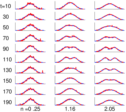
Figure 1: Time sequence of $n_{1}(z,t)$. The red line is the unsmoothed JILA data and the blue line is the numerical solution to (16). We have taken a temperature of $T=850$ nK Lewandowski2 , and the peak total density $n$ listed under each column is in units of $10^{13}$ cm^-3. We approximate $\Delta_{\mathrm{BR}}=m\omega_{\mathrm{BR}}^{2}z^{2}/2\hbar$, and take $\omega_{\mathrm{BR}}/\omega_{z}=0.09$ for each column in our calculation. This corresponds to a value $\omega_{\mathrm{diff}}/\omega_{z}=0.1$ for the first column. The axial position $z$ is in the range $\pm 600\,\mu$m.

We solved the one–dimensional spin kinetic equation (16) numerically using a finite difference scheme. For the initial state of the spin, we take $\sigma_{y}(z,p,t=0)=f_{0}(z,p),\sigma_{x}(z,p,t=0)=\sigma_{z}(z,p,t=0)=0$, corresponding to the state immediately following the first $\pi/2$ pulse. Figure 1 shows the time sequence of the density of the $|1\rangle$ state $n_{1}(z,t)=[n_{0}(z)+S_{z}(z,t)]/2$, corresponding to Fig.3(c) columns (v)-(vii) of Ref. Lewandowski . This shows that the spin segregation vanishes when the density is lowered to $n\sim 2\times 10^{12}$ cm^-3. The red curve is the raw JILA data and the blue dashed line is the theory. The agreement is striking. We also compare our numerical results to Fig.3(c) columns (i)-(iv) of Ref. Lewandowski , shown in Figure 2. In this case the density is held fixed but the curvature of the energy splitting is varied in each sequence. Note that when $\Delta_{\mathrm{BR}}(z)$ is chosen to approximately cancel $\Delta_{\mathrm{MF}}$ in the second column, the amplitude of the spin wave is essentially zero. For the larger values of $\omega_{\mathrm{diff}}$ considered in columns three and four, the agreement is only qualitative.

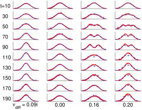
Figure 2: Time sequence of $n_{1}(z,t)$. We have taken a temperature of $T=850$ nK Lewandowski2 , and the peak total density $n$ for each column is $1.82\times 10^{13}$ cm^-3. Here, $\nu_{\mathrm{diff}}=\omega_{\mathrm{diff}}/2\pi$ is in units of Hz.

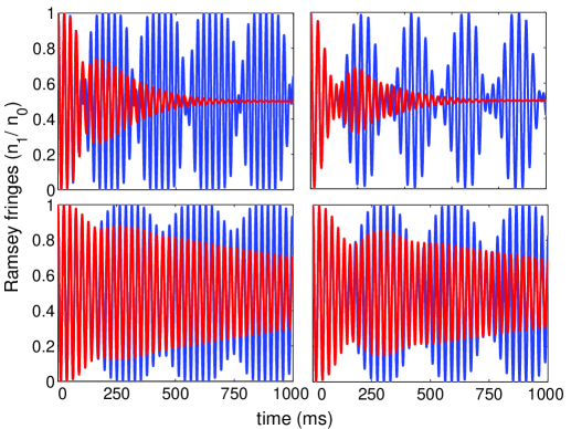
Figure 3: Modulation of Ramsey fringes. The top row corresponds to the third column of Figure 1, and in the bottom row we have set $\Delta_{\mathrm{BR}}=0$ (which corresponds to sitting at the “magic spot” bias field of 0.323 mT). The first column is taken at $z=7\,\mu$m and the second column at $z=350\,\mu$m. The red and blue lines compare the dynamics with and without collisional relaxation, respectively. We have taken a detuning of $\delta/\omega_{z}=5$.

We finally investigate the effect that the spin wave and relaxation have on the Ramsey fringes. Ramsey fringes can be obtained from the results of our calculation by simply rotating the Bloch vector $\vec{S}(z,t)$ at each time by $90^{\circ}$ about the local oscillator vector $\vec{\Omega}=\{\cos(\delta t),\sin(\delta t),0\}$, where $\delta$ is the detuning between coupling field and the hyperfine splitting. In the top row of Figure 3 we show the Ramsey fringes corresponding to the third column of Figure 1, taken at the center (left) and the edge (right) of the cloud. We compare the Ramsey fringes with (red) and without (blue) relaxation (i.e. $\left.\partial\vec{\sigma}/\partial t\right|_{1D}=0$). We find that the Ramsey fringes taken at different positions across the cloud are all modulated at the period of the spin wave, and that the fringe visibility decays when the effect of collisions is included through $\left.\partial\vec{\sigma}/\partial t\right|_{1D}$. At long times the system relaxes to the state $\vec{S}=0$, that is, the gas evolves to a completely overlapping binary mixture, which is reflected by the vanishing of the fringe visibility. In the bottom row, the differential Zeeman splitting is set to zero $\Delta_{\mathrm{BR}}=0$, which reduces the curvature of the local energy splitting. This has two main effects: the frequency of the spin wave is lowered and the fringes are visible for a much longer time. In a calculation not shown in Figure 3 for the case where the curvature is approximately zero, as in column two of Figure 2, we find that the Ramsey fringes are not modulated and do not decay, emphasizing that collisional relaxation damps out spin currents, while conserving the spin. The trends shown in the bottom row of Figure 3 agree qualitatively with experiment Lewandowski2 .

In summary, we have presented a simplified model for the spin density and current that predicts longitudinal spin waves in the gas when the energy splitting between hyperfine states in nonuniform. We have also numerically solved a one dimensional model of the Boltzmann equation that supports our simplified hydrodynamic model and gives excellent agreement with the JILA experiment Lewandowski .

While this manuscript was being written, two independent articles Oktel ; Fuchs appeared on the lanl.arXiv.org e-print archive that make predictions similar to ours.

We thank E. A. Cornell, H. J. Lewandowski, J. Roberts, and S. Rolston for useful discussions. We also thank H. J. Lewandowski for providing us the experimental data used in Fig. 1. T.N. acknowledges support from JSPS.

References

(1)
H. J. Lewandowski,
D. M. Harber,
D. L. Whitaker,
and E. A.
Cornell, cond-mat/0109476 .
(2)
A. J. Leggett and
M. J. Rice,
Phys. Rev. Lett. 20,
586 (1968).
(3)
C. Lhuillier and
F. Laloë,
J. Physique 43,
197 (1982).
(4)
L. P. Levy and
A. E. Ruckenstein,
Phys. Rev. Lett. 52,
1512 (1984).
(5)
B. R. Johnson,
J. S. Denker,
N. Bigelow,
L. P. Levy,
J. H. Freed, and
D. M. Lee,
Phys. Rev. Lett. 52,
1508 (1984).
(6)
C. Lhuiller and
F. Laloë,
J. Physique 43,
225 (1982).
(7)
C. Lhuillier,
J. Physique 44,
1 (1983).
(8)
J.-P. Bouchaud and
C. Lhuillier,
J. Physique 46,
1101 (1985).
(9)
J. Jeon and
W. Mullin,
J. Physique 49,
1691 (1988).
(10)
A. E. Ruckenstein
and L. P. Levy,
Phys. Rev. B 39,
183 (89).
(11)
H. Smith and
H. H. Jensen,
Transport Phenomena (Clarendon
Press, Oxford, 1989).
(12)
T. Nikuni and
J. E. Williams,
(unpublished).
(13)
H. J. Lewandowski,
Private communication .
(14)
M. Ö. Oktel
and L. S.
Levitov, cond-mat/011119 .
(15)
J. N. Fuchs,
D. M. Gangardt,
and F. Laloë,
cond-mat/0112228 .