Volatile Decision Dynamics: Experiments, Stochastic Description,Intermittency Control, and Traffic Optimization

The coordinated and efficient distribution of limited resources by individual decisions is a fundamental, unsolved problem. When individuals compete for road capacities, time, space, money, goods, etc., they normally make decisions based on aggregate rather than complete information, such as TV news or stock market indices. In related experiments, we have observed a volatile decision dynamics and far-from-optimal payoff distributions. We have also identified ways of information presentation that can considerably improve the overall performance of the system. In order to determine optimal strategies of decision guidance by means of user-specific recommendations, a stochastic behavioural description is developed. These strategies manage to increase the adaptibility to changing conditions and to reduce the deviation from the time-dependent user equilibrium, thereby enhancing the average and individual payoffs. Hence, our guidance strategies can increase the performance of all users by reducing overreaction and stabilizing the decision dynamics. These results are highly significant for predicting decision behaviour, for reaching optimal behavioural distributions by decision support systems, and for information service providers. One of the promising fields of application is traffic optimization.

1 Introduction

Optimal route guidance strategies in overloaded traffic networks, for example, require reliable traffic forecasts (see Fig. 1). These are extremely challenging for two reasons: First of all, traffic dynamics is very complex. However, after more than 50 years of traffic research, physicists have recently gained at least a semi-quantitative understanding of it based on the concept of self-driven, non-linearly interacting many-particle systems [2]. The second and more serious problem is the invalidation of forecasts by the driver reactions to route choice recommendations. Nevertheless, some keen scientists hope to solve this long-standing problem by means of an iteration scheme [3, 4, 5, 6, 7, 8, 9, 10, 11]: If the driver reaction was known from experiments [12, 13, 14, 15, 16, 17, 18, 19, 20, 21, 22], the resulting traffic situation could be calculated, yielding improved route choice recommendations, etc. Given this iteration scheme converges, it would facilitate optimal recommendations and reliable traffic forecasts anticipating the driver reactions. Based on empirically determined transition and compliance probabilities, we will develop a new procedure in the following, which would even allow us to reach the optimal traffic distribution in one single step and in harmony with the forecast.

Figure 1: Schematic illustration of a day-to-day route choice scenario. Each day, the drivers have to decide between two alternative routes, 1 and 2. Note that, due to the different number of lanes, route 1 has a higher capacity than route 2. The latter is, therefore, used by less cars.

The solution of this difficult and practically relevant problem requires several concepts and methods from physics. First of all, we will identify the essential role and reason of intermittency in scenarios with repeated decisions (see Sec. 3). Second, we will derive a non-linear feedback mechanism for intermittency control (see Sec. 4). In addition, we will develop a stochastic description of the decision behavior (see Sec. 5) and evaluate the corresponding transition and compliance probabilities including their time-dependence (see Sec. 4).

2 Experimental setup and previous results

Figure 2: Schematic illustration of the decision experiment. Several test persons have to take decisions based on the aggregate information their computer displays. The computers are connected and can, therefore, exchange information. However, a direct communication among players is suppressed.

To determine the route choice behavior, Schreckenberg, Selten et al. [19] have recently carried out a decision experiment [1] (see Fig. 2). $N$ test persons had to repeatedly decide between two alternatives $1$ and $2$ (the routes) and should try to maximize their resulting payoffs (describing something like the speeds or inverse travel times). To reflect the competition for a limited resource (the road capacity), the received payoffs

$$P_{1}(n_{1})=P_{1}^{0}-P_{1}^{1}n_{1}\quad\mbox{and}\quad P_{2}(n_{2})=P_{2}^{0}-P_{2}^{1}n_{2}$$ (1)

went down with the numbers of test persons $n_{1}$ and $n_{2}=N-n_{1}$ deciding for alternatives 1 and 2, respectively. The user equilibrium corresponding to equal payoffs for both alternative decisions is found for a fraction

$$f_{1}^{\rm eq}=\frac{n_{1}}{N}=\frac{P_{2}^{1}}{P_{1}^{1}+P_{2}^{1}}+\frac{1}{N}\frac{P_{1}^{0}-P_{2}^{0}}{P_{1}^{1}+P_{2}^{1}}$$ (2)

of persons choosing alternative 1. The system optimum corresponds to the maximum of the total payoff $n_{1}P_{1}(n_{1})+n_{2}P_{2}(n_{2})$, which lies by an amount of

$$\frac{1}{2N}\frac{P_{1}^{0}-P_{2}^{0}}{P_{1}^{1}+P_{2}^{1}}$$ (3)

below the user optimum. Therefore, only experiments with a few players allow to find out, whether the test persons adapt to the user or the system optimum. Small groups are also more suitable for the experimental investigation of the fluctuations in the system and of the long-term adaptation behavior. Schreckenberg, Selten et al. found that, on average, the test groups adapted relatively well to the user equilibrium. However, although it appears reasonable to stick to the same decision once the equilibrium is reached, the standard deviation stayed at a finite level. This was not only observed in “treatment” 1, where all players knew only their own (previously experienced) payoff, but also in treatment 2, where the payoffs $P_{1}(n_{1})$ and $P_{2}(n_{2})$ for both, 1- and 2-decisions, were transmitted to all players (analogous to radio news). Nevertheless, treatment 2 could decrease the changing rate and increase the average payoffs. For details regarding the statistical analysis see Ref. [19].

Figure 3: Overview of treatments 1 to 5 (with $N=9$ and payoff parameters $P_{2}^{0}=28$, $P_{1}^{1}=4$, $P_{2}^{1}=6$, and $P_{1}^{0}=34$ for $0\leq t\leq 1500$, but a zick-zack-like variation between $P_{1}^{0}=44$ and $P_{1}^{0}=-6$ with a period of $50$ for $1501\leq t\leq 2500$): (a) Average number of decisions for alternative 1 (solid line) compared to the user equilibrium (dashed line), (b) standard deviation of the number of 1-decisions from the user equilibrium, (c) number of decision changes from one iteration to the next one, (d) average payoff per iteration for players who have changed their decision and for all players. The latter increased with a reduction in the changing rate, but normally stayed below the payoff in the user equilibrium (which is 1 on average in treatments 4 and 5, otherwise 10). The displayed moving time-averages [(a) over 40 iterations, (b)-(d) over 100 iterations] illustrate the systematic response to changes in the treatment every 500 iterations. Dashed lines in (b)-(d) show estimates of the stationary values after the transient period (to guide the eyes), while time periods around the dotted lines are not significant. Compared to treatment 1, treatment 3 managed to reduce the changing rate and to increase the average payoffs (three times more than treatment 2 did). These changes were systematic for all players (see Fig. 4). In treatment 4, the changing rate and the standard deviation went up, since the user equilibrium changed in time. The user-specific recommendations in treatment 5 could almost fully compensate for this. The above conclusions are also supported by additional experiments with single treatments.

To explain the mysterious persistence in the changing behavior and explore possibilities to suppress it, we have repeated these experiments with more iterations and tested additional treatments. In the beginning, all treatments were consecutively applied to the same players in order to determine the response to different kinds of information (see Fig. 3). Afterwards, single treatments and variants of them have been repeatedly tested with different players to check our conclusions. Apart from this, we have generalized the experimental setup in the sense that it was not anymore restricted to route choice decisions: The test persons did not have any idea of the payoff functions in the beginning, but had to develop their own hypothesis about them. In particular, the players did not know that the payoff decreased with the number of persons deciding for the same alternative.

Figure 4: Comparison of the individual decision behaviors under (a) treatment 1, (b) treatment 2, and (c) treatment 3. The upper values correspond to a decision for alternative 2, the lower ones for alternative 1. Note that some test persons showed similar behaviors (either more or less the same or almost opposite ones), although they could not talk to each other. This shows that there are some typical strategies how to react to specific information. The group has, in fact, to develop complementary strategies in order to reach a good adaptation performance. Identical strategies would perform poorly (as in the minority game [23, 24, 25, 26]). Despite the mentioned complementary behavior, there is a characteristic reaction to changes in the treatment. For example, compared to treatment 2 all players reduce their changing rate in treatment 3.

In treatment 3, every test person was informed about the own payoff $P_{1}(n_{1})$ [or $P_{2}(n_{2})$] and the potential payoff

$$P_{2}(N-n_{1}+\epsilon N)=P_{2}(n_{2})-\epsilon NP_{2}^{1}$$ (4)

[or $P_{1}(N-n_{2}+\epsilon N)=P_{1}(n_{1})-\epsilon NP_{1}^{1}$] he or she would have obtained, if a fraction $\epsilon$ of persons had additionally chosen the other alternative (here: $\epsilon=1/N=1/9$). Treatments 4 and 5 were variants of treatment 3, but some payoff parameters were changed in time to simulate varying environmental conditions. In treatment 5, each player additionally received an individual recommendation which alternative to choose.

The higher changing rate in treatment 1 compared to treatment 2 can be understood as effect of an exploration rate $\nu_{1}$ required to find out which alternative performs better. It is also plausible that treatment 3 could further reduce the changing rate: In the user equilibrium with $P_{1}(n_{1})=P_{2}(n_{2})$, every player knew that he or she would not get the same, but a reduced payoff, if he or she would change the decision. That explains why the new treatment 3 could reach a great adaptation performance, reflected by a very low standard deviation and almost optimal average payoffs. The behavioral changes induced by the treatments were not only observed on average, but for every single individual (see Fig. 4). Moreover, even the smallest individual cumulative payoff exceeded the highest one in treatment 1. Therefore, treatment 3’s way of information presentation is much superior to the ones used today.

3 Explaining the volatile decision dynamics

In this section, we will investigate why players changed their decision in the user equilibrium at all. The reason for the pertaining changing behavior can be revealed by a more detailed analysis of the individual decisions in treatment 3. Figure 5 shows some kind of intermittent behavior, i.e. quiescent periods without changes, followed by turbulent periods with many changes. This is reminiscent of volatility clustering in stock market indices [27, 28, 29], where individuals also react to aggregate information reflecting all decisions (the trading transactions). Single players seem to change their decision to reach above-average payoffs. In fact, although the cumulative individual payoff is anticorrelated with the average changing rate, some players receive higher

Figure 5: Illustration of typical results for treatment 3 (which was here the only treatment applied to the test persons, in contrast to Fig. 3). (a) Decisions of all 9 players. Players are displayed from the top to the bottom in the order of increasing changing rate. Although the ranking of the cumulative payoff and the changing rate are anticorrelated, the relation is not monotonic. Note that turbulent or volatile periods characterized by many decision changes are usually triggered by individual changes after quiescent periods (dotted lines). (b) The changing rate is mostly larger than the (standard) deviation from the user equilibrium $n_{1}=f_{1}^{\rm eq}N=6$, indicating an overreaction in the system.

payoffs with larger changing rates than others. They profit from the overreaction in the system. Once the system is out of equilibrium, all players respond in one way or another. Typically, there are too many decision changes (see Figs. 5 and 6). The corresponding overcompensation, which had also been predicted by computer simulations [5, 8, 9, 10, 17, 30], gives rise to “turbulent” periods.

We should, however, note that the calm periods without decision changes tend to become longer in the course of time. That is, after a very long time period the individuals learn not to change their behavior when the user equilibrium is reached. This is not only found in Fig. 5, but also visible in Fig. 3c after about 800 iterations. In larger systems (with more participants) this transient period would take even longer, so that this stabilization effect cannot be observed in experiments with less iterations or more test persons.

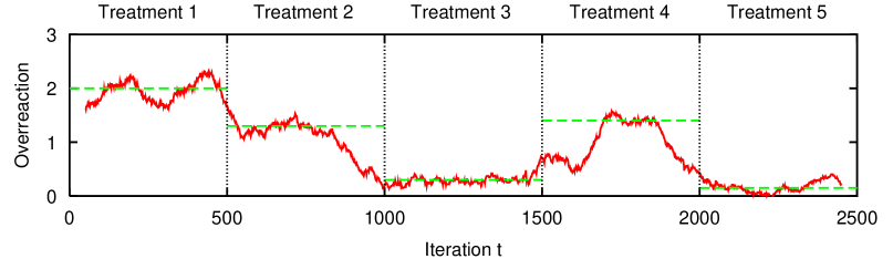
Figure 6: Measured overreaction, i.e., difference between the actual number of decision changes (the changing rate) and the required one (the standard deviation). The overreaction can be significantly influenced by the treatment, i.e. the way of information presentation. The minimum overreaction was reached by treatment 5, i.e. user-specific recommendations.

Finally, we should stress that other interpretations of the rather persistent decision changes have been ruled out, for example, an unstable user equilibrium or a competition between the user optimum and the system optimum. High changing rates also occur if the user and system equilibrium agree, and if the payoff functions $P_{1}(n_{1})$ and $P_{2}(n_{2})$ are the same (i.e. $f_{1}^{\rm eq}=1/2$).

4 Decision and intermittency control by non-linear feedback based on guidance strategies

To avoid overreaction, in treatment 5 we have recommended a number $f_{1}^{\rm eq}(t+1)N-n_{1}(t)$ of players to change their decision and the other ones to keep it. These user-specific recommendations helped the players to reach the smallest overreaction of all treatments (see Fig. 6) and a very low standard deviation, although the payoffs were changing in time (see Fig. 7). Treatment 4 shows how the group performance was affected by the time-dependent user equilibrium: Even without recommendations, the group managed to adapt to the changing conditions surprisingly well, but the standard deviation and changing rate were approximately as high as in treatment 2 (see Fig. 3). This adaptability (the collective “group intelligence”) is based on complementary responses (direct and contrary ones [19], “movers” and “stayers”, cf. Fig. 4). That is, if some players do not react to the changing conditions, others will take the chance to earn additional payoff. This experimentally supports the behavior assumed in the theory of efficient markets, but here the efficiency is limited by overreaction.

Figure 7: Representative examples for (a) treatment 4 and (b) treatment 5. The displayed curves are moving time-averages over 20 iterations. Compared to treatment 4, the user-specific recommendations in treatment 5 (assuming $C_{M}=C_{S}=1$, $R_{1}=0$, $R_{2}=\max([f_{1}^{\rm eq}(t+1)N-n_{1}(t)+B(t+1)]/n_{2}(t),1)$, $I_{1}=I_{2}=1$) could increase the group adaptability to the user equilibrium a lot, even if they had a systematic or random bias $B$ (see Fig. 8a). The standard deviation was reduced considerably and the changing rate even more.

In most experiments, we found a constant and high compliance $C_{S}(t)\approx 0.92$ with recommendations to stay, but the compliance $C_{M}(t)$ with recommendations to change (to ‘move’) [15, 16, 31, 32] turned out to vary in time. It decreased with the reliability of the recommendations (see Fig. 8a), which again dropped with the compliance.

Figure 8: (a) In treatment 5, the compliance to recommendations to change dropped considerably below the compliance to recommendations to stay. The compliance to changing recommendations was very sensitive to the degree of their reliability, i.e. participants followed recommendations just as much as they helped them to reach the user equilibrium (so that the bias $B$ did not affect the small deviation from it, see Fig. 7b). While during time interval A, the recommendations would have been perfect, if all players had followed them, in time interval B the user equilibrium was overestimated by $B=+1$, in C it was underestimated by $B=-2$, in D it was randomly over- or underestimated by $B=\pm 1$, and in E by $B=\pm 2$. Obviously, a random error is more serious than a systematic one of the same amplitude. Dotted non-vertical lines illustrate the estimated compliance levels during the transient periods and afterwards (horizontal dotted lines). (b) The average payoffs varied largely with the decision behavior. Players who changed their decision got significantly lower payoffs on average than those who kept their previous decision. Even recommendations could not overcome this difference: It stayed profitable not to change, although it was generally better to follow recommendations than to refuse them. For illustrative reasons, the third and fourth line were shifted by 15, while the fifth and sixth line were shifted by 30 iterations.

Based on this knowledge, we have developed a model, how the competition for limited resources (such as road capacity) could be optimally guided by means of information services. Let us assume we had $n_{1}(t)$ 1-decisions at time $t$, but the optimal number of 1-decision at time $t+1$ is calculated to be $f_{1}^{\rm eq}(t+1)N\geq n_{1}(t)$. Our aim is to balance the deviation $f_{1}^{\rm eq}(t+1)N-n_{1}(t)\geq 0$ by the expected net number

$$\langle\Delta n_{1}(t+1)\rangle=\langle n_{1}(t+1)-n_{1}(t)\rangle=\langle n_{1}(t+1)\rangle-n_{1}(t)$$ (5)

of transitions from decision 2 to decision 1, i.e. $f_{1}^{\rm eq}(t+1)N-n_{1}(t)=\langle\Delta n_{1}(t+1)\rangle$. In the case $f_{1}^{\rm eq}(t+1)N-n_{1}(t)<0$, indices 1 and 2 have to be interchanged.

Let us assume we give recommendations to fractions $I_{1}(t)$ and $I_{2}(t)$ of players who had chosen decision 1 and 2, respectively. The fraction of changing recommendations to previous 1-choosers shall be denoted by $R_{1}(t)$, and for previous 2-choosers by $R_{2}(t)$. Correspondingly, fractions of $[1-R_{1}(t)]$ and $[1-R_{2}(t)]$ receive a recommendation to stick to the previous decision. Moreover, $[1-C_{M}(t)]$ is the refusal probability of recommendations to change, while $[1-C_{S}(t)]$ is the refusal probability of recommendations to stay. Finally, we denote the spontaneous transition probability from decision 1 to 2 by $p_{a}(2|1,n_{1};t)$ and the inverse transition probability by $p_{a}(1|2,n_{1};t)$, in case a player does not receive any recommendation. This happens with probabilities $[1-I_{1}(t)]$ and $[1-I_{2}(t)]$, respectively. Both transition probabilities $p_{a}(2|1,n_{1};t)$ and $p_{a}(1|2,n_{1};t)$ are functions of the number $n_{1}(t)=N-n_{2}(t)$ of previous 1-decisions. The index $a$ allows us to reflect different strategies or characters of players. The fraction of players pursuing strategy $a$ is then denoted by $F_{a}(t)$. Applying methods summarized in Ref. [33], the expected change $\langle\Delta n_{1}(t+1)\rangle$ of $n_{1}$ is given by the balance equation

$$\langle\Delta n_{1}(t+1)\rangle = \sum_{a}p_{a}(1|2,n_{1};t)F_{a}(t)[1-I_{2}(t)]n_{2}(t)$$ (6)

$$- \sum_{a}p_{a}(2|1,n_{1};t)F_{a}(t)[1-I_{1}(t)]n_{1}(t)$$

$$+ \sum_{a}\{C_{M}^{a}(t)R_{2}(t)+[1-C_{S}^{a}(t)][1-R_{2}(t)]\}F_{a}(t)I_{2}(t)n_{2}(t)$$

$$- \sum_{a}\{C_{M}^{a}(t)R_{1}(t)+[1-C_{S}^{a}(t)][1-R_{1}(t)]\}F_{a}(t)I_{1}(t)n_{1}(t)\,.\quad$$

Together with the requirement

$$\langle\Delta n_{1}(t+1)\rangle=f_{1}^{\rm eq}(t+1)N-n_{1}(t)\,,$$ (7)

this equation defines, with respect to the number $n_{1}$ of previous 1-decisions, a non-linear feedback or control strategy.

Note that, for Eq. (6), it was not necessary to distinguish different characters $a$. We have, therefore, evaluated the overall transition probabilities

$$p(1|2,n_{1};t)=\sum_{a}p_{a}(1|2,n_{1};t)F_{a}(t)\quad\mbox{and}\quad p(2|1,n_{1};t)=\sum_{a}p_{a}(2|1,n_{1};t)F_{a}(t)\,.$$ (8)

According to classical decision theories [33, 34, 35, 36], we would expect that the transition probabilities $p_{a}(1|2,n_{1};t)$ and $p(1|2,n_{1};t)$ should be monotonically increasing functions of the payoff $P_{1}(n_{1}(t))$, the payoff difference $P_{1}(n_{1}(t))-P_{2}(N-n_{1}(t))$, the potential payoff $P_{1}(n_{1}(t)+\epsilon N)$, or the potential payoff gain $P_{1}(n_{1}(t)+\epsilon N)-P_{2}(N-n_{1}(t))$. All these quantities vary linearly with $n_{1}$, so that $p(1|2,n_{1};t)$ should be a monotonic function of $n_{1}(t)$. A similar thing should apply to $p(2|1,n_{1};t)$. Instead, the experimental data point to transition probabilities with a minimum at the user equilibrium (see Fig. 9a). That is, the players stick to a certain alternative for a longer time, when the system is close to the user equilibrium. This is a result of learning [37] (see also Refs. [38, 39, 40, 41, 42]). In fact, we find a gradual change of the transition probabilities in time (see Fig. 9b). The corresponding “learning curves” reflect the players’ adaptation to the user equilibrium.

Figure 9: Illustration of decision distributions $P(i|n_{1})$ and transition probabilities $p(i^{\prime}|i,n_{1};t)$ measured in treatment 3. (a) The probability $P(1|n_{1})$ to choose alternative 1 was approximately 2/3, independently of the number $n_{1}$ of players who had previously chosen alternative 1. The probability $P(2|n_{1})$ to choose alternative 2, given that $n_{1}$ players had chosen alternative 1, was always about 1/3. In contrast, the transition probability $p(1|2,n_{1})$ describing decision changes from alternative 2 to 1 did depend on the number $n_{1}$ of players who had chosen decision 1. The same was true for the inverse transition probability $p(2|1,n_{1})$ from decision 1 to decision 2. Remarkably enough, these transition probabilities are not monotonically increasing with the payoff or the expected payoff gain, as they do not monotonically increase with $n_{1}$. Instead, the probability to change the decision shows a minimum at the user equilibrium $n_{1}=f_{1}^{\rm eq}N=6$. (b) The reason for the different transition probabilities is an adaptation process in which the participants learn to take fewer changing decisions, when the user equilibrium is reached or close by, but more, when the user equilibrium is far away. (The curves were exponentially smoothed with $\alpha=0.05$.)

After the experimental determination of the transition probabilities $p(2|1,n_{1};t)$, $p(1|2,n_{1};t)$ and specification of the overall compliance probabilities

$$C_{M}(t)=\sum_{a}C_{M}^{a}(t)F_{a}(t)\,,\qquad C_{S}(t)=\sum_{a}C_{S}^{a}(t)F_{a}(t)\,,$$ (9)

we can guide the decision behavior in the system via the levels $I_{i}(t)$ of information dissemination and the fractions $R_{i}(t)$ of recommendations to change ($i\in\{1,2\}$). These four degrees of freedom allow us to apply a variety of guidance strategies depending on the respective information medium. For example, a guidance by radio news is limited by the fact that $I_{1}(t)=I_{2}(t)$ is given by the average percentage of radio users. Therefore, equations (6) and (7) cannot always be solved by variation of the fractions of changing recommendations $R_{i}(t)$. User-specific services have much higher guidance potentials and could, for example, be transmitted via SMS. Among the different guidance strategies fulfilling equations (6) and (7), the one with the minimal statistical variance will be the best. However, it would already improve the present situation to inform everyone about the fractions $R_{i}(t)$ of participants who should change their decision, as users can learn to respond with varying probabilities (see Fig. 9).

The outlined guidance strategy could, of course, also be applied to reach the system optimum rather than the user optimum. The values of $\Delta n_{1}(t+1)$ would just be different. Note, however, that the users would soon recognize that this guidance is not suitable to reach the user optimum. Consequently, the compliance probabilities $C_{j}(t)$ with $j\in\{M,S\}$ would gradually go down, which would affect the potentials and reliability of the guidance system. This problem can only be solved by a suitable modification of the payoff functions, adapting the user optimum to the system optimum.

In practical applications, we would determine the time-dependent compliance probabilities $C_{j}(t)$ (and the transition probabilities) on-line with an exponential smoothing procedure according to

$$C_{j}(t+1)=\alpha C^{\prime}_{j}(t)+(1-\alpha)C_{j}(t)\quad\mbox{with}\quad\alpha\approx 0.1\,,$$ (10)

where $C^{\prime}_{j}(t)$ is the percentage of participants who have followed their recommendation at time $t$. As the average payoff for decision changes is normally lower than for staying with the previous decision (see Figs. 8b and 3d), a high compliance probability $C_{M}$ is hard to achieve. That is, individuals who follow recommendations to change normally pay for reaching the user equilibrium (because of the overreaction in the system). Hence, there are no good preconditions to charge the players for recommendations, as we did in another treatment. Consequently, only a few players requested recommendations, which reduced their reliability, so that the overall performance of the system went down.

5 Master equation description of iterated decisions

The stochastic description of decisions that are taken at discrete time steps (e.g. on a day-to-day basis) is possible by means of the time-discrete master equation [2]

$$P(\mathchoice{\mbox{\boldmath$\displaystyle n$}}{\mbox{\boldmath$\textstyle n$}}{\mbox{\boldmath$\scriptstyle n$}}{\mbox{\boldmath$\scriptscriptstyle n$}},t+\Delta t)=\sum_{\mathchoice{\mbox{\boldmath$\displaystyle n$}}{\mbox{\boldmath$\textstyle n$}}{\mbox{\boldmath$\scriptstyle n$}}{\mbox{\boldmath$\scriptscriptstyle n$}}^{\prime}}P(\mathchoice{\mbox{\boldmath$\displaystyle n$}}{\mbox{\boldmath$\textstyle n$}}{\mbox{\boldmath$\scriptstyle n$}}{\mbox{\boldmath$\scriptscriptstyle n$}},t+\Delta t|\mathchoice{\mbox{\boldmath$\displaystyle n$}}{\mbox{\boldmath$\textstyle n$}}{\mbox{\boldmath$\scriptstyle n$}}{\mbox{\boldmath$\scriptscriptstyle n$}}^{\prime},t)P(\mathchoice{\mbox{\boldmath$\displaystyle n$}}{\mbox{\boldmath$\textstyle n$}}{\mbox{\boldmath$\scriptstyle n$}}{\mbox{\boldmath$\scriptscriptstyle n$}}^{\prime},t)$$ (11)

with $\Delta t=1$ unit time. Herein, $P(\mathchoice{\mbox{\boldmath$\displaystyle n$}}{\mbox{\boldmath$\textstyle n$}}{\mbox{\boldmath$\scriptstyle n$}}{\mbox{\boldmath$\scriptscriptstyle n$}},t)$ denotes the occurence probability of the configuration $\mathchoice{\mbox{\boldmath$\displaystyle n$}}{\mbox{\boldmath$\textstyle n$}}{\mbox{\boldmath$\scriptstyle n$}}{\mbox{\boldmath$\scriptscriptstyle n$}}=(n_{1},n_{2})$ at time $t$. This vector comprises the occupation numbers $n_{i}$ and reflects the decision distribution in the system. As the number of individuals changing to the other alternative is given by a binomial distribution, we obtain the following expression for the configurational transition probability:

$$P\big{(}(n_{1},n_{2}),t+1\,\big{|}\,(n_{1}-\Delta n_{1},n_{2}+\Delta n_{1}),t\big{)}$$

$$\quad=\!\!\!\sum_{k=0}^{\min(n_{1}-\Delta n_{1},n_{2})}\left(\begin{array}[]{c}n_{2}+\Delta n_{1}\\ \Delta n_{1}+k\end{array}\right)p(1|2,n_{1}-\Delta n_{1};t)^{\Delta n_{1}+k}\big{[}1-p(1|2,n_{1}-\Delta n_{1};t)\big{]}^{n_{2}-k}$$ (14)

$$\quad\qquad\times\left(\begin{array}[]{c}n_{1}-\Delta n_{1}\\ k\end{array}\right)p(2|1,n_{1}-\Delta n_{1};t)^{k}\big{[}1-p(2|1,n_{1}-\Delta n_{1};t)\big{]}^{n_{1}-\Delta n_{1}-k}\,.$$ (17)

This formula sums up the probabilities that $\Delta n_{1}+k$ of $n_{2}+\Delta n_{1}$ previous 2-choosers change independently to alternative 1 with probability $p(1|2,n_{1}-\Delta n_{1};t)$, while $k$ of the $n_{1}-\Delta n_{1}$ previous 1-choosers change to alternative 2 with probability $p(2|1,n_{1}-\Delta n_{1};t)$, so that the net number of changes is $\Delta n_{1}$. If $\Delta n_{1}<0$, the roles of alternatives 1 and 2 have to be interchanged. Formulas (11) and (17) would look even more compicated, if we distinguished several characters $a$. We would, then, have to replace the binomial distributions by multinomial ones.

The potential use of Eq. (17) is the calculation of the statistical variation of the decision distribution or, equivalently, the number $n_{1}$ of 1-choosers. It also allows one to determine the variance, which the optimal guidance strategy should minimize in favour of reliable recommendations.

6 Summary and Outlook

In this contribution, we have discovered that the dynamics of iterated decisions based on aggregate information is intermittent. In order to control intermittency, we have developed a stochastic description and a non-linear feedback mechanism. That is, the application of several physical concepts and methods allowed us to gain a detailled understanding of decision dynamics, which is required for practical applications.

In more detail, we have explored different and identified superior ways of information presentation that facilitate to guide user decisions in the spirit of higher payoffs. By far the least standard deviations from the user equilibrium could be reached by presenting the own payoff and the potential payoff, if the respective participant (or a certain fraction of players) had additionally chosen the other alternative. Interestingly, the decision dynamics was found to be intermittent similar to the volatility clustering in stock markets, where individuals also react to aggregate information. This results from the desire to reach above-average payoffs, combined with the immanent overreaction in the system. We have also demonstrated that payoff losses due to a volatile decision dynamics (e.g., excess travel times) can be reduced via user-specific recommendations by a factor of three or more. Such kinds of results will be applied to the route guidance on German highways (see, for example, the project SURVIVE conducted by Nobel prize winner Reinhard Selten and Michael Schreckenberg). Optimal recommendations to reach the user equilibrium follow directly from the derived balance equations (6) and (7) for decision changes based on empirical transition and compliance probabilities. The quantification of the transition probabilities needs a novel stochastic description of the decision behavior, which is not just driven by the potential (gains in) payoffs, in contrast to intuition and established models. To understand these findings, one has to take into account individual learning.

Obviously, it requires both, theoretical and experimental efforts to get ahead in decision theory. In a decade from now, the theory of “elementary” human interactions will probably have been developed to a degree that allows one to systematically derive social patterns and economic dynamics on this ground in a similar way as the structure, properties, and dynamics of matter have been derived from elementary physical interactions. This will not only yield a deeper understanding of socio-economic systems, but also help to more efficiently distribute scarce resources such as road capacities, time, space, money, energy, goods, or our natural environment. One day, similar guidance strategies as the ones suggested above may help politicians and managers to stabilize economic markets, to increase average and individual profits, and to decrease the unemployment rate. Physics can contribute to this goal, in particular with the methods developed in the fields of non-linear dynamics and statistical physics.

Acknowledgment: The authors are grateful to the ALTANA-Quandt foundation for financial support, to Tilo Grigat for preparing some of the illustrations, and to the test persons.

References

- [1] J. H. Hagel and A. E. Roth (Eds.), The Handbook of Experimental Economics (Princeton University, Princeton, NJ, 1995).
- [2] D. Helbing, Traffic and related self-driven many-particle systems, Reviews of Modern Physics 73, 1067-1141 (2001).
- [3] M. Schreckenberg and R. Selten (Eds.), Human Behaviour and Traffic Networks (Springer, Berlin, 2002), to appear.
- [4] M. Ben-Akiva, J. Bottom, and M. S. Ramming, Route guidance and information systems, Int. J. Syst. Contr. Engin. 215, 317-324 (2001).
- [5] W. Barfield and T. Dingus, Human Factors in Intelligent Transportation Systems (Erlbaum, Mahwah, NJ, 1998).
- [6] J. Wahle, A. Bazzan, F. Klügl, and M. Schreckenberg, Decision dynamics in a traffic scenario, Physica A 287, 669-681 (2000).
- [7] Articles in Route Guidance and Driver Information, IEE Conference Publications, Vol. 472 (IEE, London, 2000).
- [8] M. Ben-Akiva, A. de Palma, and I. Kaysi, Dynamic network models and driver information systems, Transportation Research A 25, 251-266 (1991).
- [9] H. S. Mahmassani and R. Jayakrishnan, System performance and user response under real-time information in a congested traffic corridor, Transportation Research A 25, 293-307 (1991).
- [10] R. Arnott, A. de Palma, and R. Lindsey, Does providing information to drivers reduce traffic congestion?, Transportation Research A 25, 309-318 (1991).
- [11] J. Adler and V. Blue, Towards the design of intelligent traveler information systems, Transportation Research C 6, 157-172 (1998).
- [12] H. S. Mahmassani and R. C. Jou, Transferring insights into commuter behavior dynamics from laboratory experiments to field surveys, Transportation Research A 34, 243-260 (2000).
- [13] P. Bonsall, P. Firmin, M. Anderson, I. Palmer, and P. Balmforth, Validating the results of a route choice simulator Transportation Research C 5, 371-387 (1997).
- [14] Y. Iida, T. Akiyama, and T. Uchida, Experimental analysis of dynamic route choice behavior, Transportation Research B 26, 17-32 (1992).
- [15] P. S.-T. Chen, K. K. Srinivasan, and H. S. Mahmassani, Effect of information quality on compliance behavior of commuters under real-time traffic information, Transportation Research Record 1676, 53-60 (1999).
- [16] R. D. Kühne, K. Langbein-Euchner, M. Hilliges, and N. Koch, Evaluation of compliance rates and travel time calculation for automatic alternative route guidance systems on freeways., Transportation Research Record 1554, 153-161 (1996).
- [17] R. Hall, Route choice and advanced traveler information systems on a capacitated and dynamic network, Transportation Research C 4, 289-306 (1996).
- [18] A. Khattak, A. Polydoropoulou, and M. Ben-Akiva, Modeling revealed and stated pretrip travel response to advanced traveler information systems, Transportation Research Record 1537, 46-54 (1996).
- [19] M. Schreckenberg, R. Selten, T. Chamura, T. Pitz, and J. Wahle, Experiments on day-to-day route choice (and references therein), e-print www.trafficforum.org/01080701, submitted to Cooper@tive Tr@nsport@tion Dyn@mics (2001).
- [20] H. N. Koutsopoulos, A. Polydoropoulou, and M. Ben-Akiva, Travel simulators for data collection on driver behavior in the presence of information, Transportation Research C 3, 143-159 (1995).
- [21] H. S. Mahmassani, and D.-G. Stephan, Experimental investigation of route and departure time choice dynamics of urban commuters. Transportation Research Records 1203, 69-84 (1988).
- [22] P. Bonsall, The influence of route guidance advice on route choice in urban networks, Transportation 19, 1-23 (1992).
- [23] W. B. Arthur, Inductive reasoning and bounded rationality, American Econonmic Review 84, 406-411 (1994).
- [24] D. Challet and Y.-C. Zhang, Emergence of cooperation and organization in an evolutionary game, Physica A 246, 407ff (1997).
- [25] D. Challet and Y.-C. Zhang, On the minority game: Analytical and numerical studies, Physica A 256, 514-532 (1998).
- [26] D. Challet, M. Marsili, and Y.-C. Zhang, Modeling market mechanism with minority game Physica A 276, 284-315 (2000).
- [27] R. N. Mantegna, and H. E. Stanley, Introduction to Econophysics: Correlations and Complexity in Finance (Cambridge University, Cambridge, England, 1999).
- [28] S. Ghashghaie, W. Breymann, J. Peinke, P. Talkner, and Y. Dodge, Turbulent cascades in foreign exchange markets, Nature 381, 767-770 (1996).
- [29] T. Lux and M. Marchesi, Scaling and criticality in a stochastic multi-agent model of a financial market, Nature 397, 498-500 (1999).
- [30] J. Wahle, A. L. C. Bazzan, F. Klügl, and M. Schreckenberg, Anticipatory traffic forecast using multi-agent techniques, in Traffic and Granular Flow ’99, pp. 87-92, D. Helbing, H. J. Herrmann, M. Schreckenberg, and D. E. Wolf (Eds.) (Springer, Berlin, 2000).
- [31] M. Kraan, H. S. Mahmassani, and N. Huynh, Traveler responses to advanced traveler information systems for shopping trips: Interactive survey approach, Transportation Research Record 1725, 116 (2000).
- [32] K. K. Srinivasan and H. S. Mahmassani, Modeling inertia and compliance mechanisms in route choice behavior under real-time information, Transportation Research Record 1725, 45-53 (2000).
- [33] D. Helbing, Quantitative Sociodynamics (and references therein) (Kluwer Academic, Dordrecht, 1995).
- [34] J. de D. Ortúzar and L. G. Willumsen, Modelling Transport, Chap. 7: Discrete-Choice Models (Wiley, Chichester, 1990).
- [35] M. Ben-Akiva, D. M. McFadden et al., Extended framework for modeling choice behavior, Marketing Letters 10, 187-203 (1999).
- [36] M. Ben-Akiva and S. R. Lerman, Discrete Choice Analysis: Theory and Application to Travel Demand (MIT Press, Cambridge, MA, 1997).
- [37] S. Nakayama and R. Kitamura, Route choice model with inductive learning, Transportation Research Record 1725, 63-70 (2000).
- [38] Y.-W. Cheung and D. Friedman, Individual learning in normal form games: Some laboratory results, Games and Economic Behavior 19(1), 46-76 (1997).
- [39] I. Erev and A. E. Roth, Predicting how people play games: Reinforcement learning in experimental games with unique, mixed strategy equilibria, American Economic Review 88(4), 848-881 (1998).
- [40] J. Nachabar, Prediction, optimization, and learning in repeated games, Econometrica 65, 275-309 (1997).
- [41] J. B. van Huyck, R. C. Battlio, and R. O. Beil, Tacit coordination games, strategic uncertainty, and coordination failure, American Economic Review 80(1), 234-252 (1990).
- [42] J. B. van Huyck, J. P. Cook, and R. C. Battlio, Selection dynamics, asymptotic stability, and adaptive behavior, Journal of Political Economy 102(5), 975-1005 (1994).