Tunneling effect on composite fermion pairing state in bilayer quantum Hall system

Takao Morinari
Abstract

We discuss the composite fermion pairing state in bilayer quantum Hall systems. After the evaluation of the range of the inter-layer separation in which the quantum Hall state is stabilized, we discuss the effect of inter-layer tunneling on the composite fermion pairing state at $\nu=1/2$. We show that there is a cusp at the transition point between the Halperin $(3,3,1)$ state and the Pfaffian state.

73.40.Hm, 71.10.Pm

I Introduction

As a remarkable example of strongly correlated electron systems, the fractional quantum Hall effect has been studied extensively.[1, 2] In the fractional quantum Hall systems, the Coulomb interaction plays a dominant role. Due to the presence of the strong magnetic field, the Coulomb interaction gives rise to a two-body correlation of non-zero relative angular momentum. The Laughlin wave function,[3] which captures the essential properties of the system, consists of this two-body correlation only. The role of the Coulomb interaction to generate the two-body correlation becomes clear when it is described in terms of Haldane’s pseudopotential.[4] From the analysis of the pseudopotentials, one can see that the most fundamental contribution comes from the short-range Coulomb interaction.

In the single-layer quantum Hall systems, it is hard to change the short-range Coulomb interaction. Whereas in the bilayer quantum Hall systems, we can adjust the inter-layer Coulomb interaction by varying the inter-layer separation $d$. In addition, there is another parameter, the inter-layer tunneling amplitude $t$ to control the system. Since there are such additional parameters to control the system, we can expect rich phase diagram in the bilayer quantum Hall systems.

In the absence of inter-layer tunneling, the properties of the system seems to be well described by the Halperin $(m,m,n)$ wave function[5], which is an extention of the Laughlin wave function:

$\displaystyle\Psi_{mmn}(z_{1}^{\uparrow},z_{2}^{\uparrow},\cdots,z_{N}^{\uparrow};z_{1}^{\downarrow},z_{2}^{\downarrow},\cdots,z_{N}^{\downarrow})$ (1)
$\displaystyle=$ $\displaystyle\prod_{i<j}(z_{i}^{\uparrow}-z_{j}^{\uparrow})^{m}\prod_{i<j}(z_{i}^{\downarrow}-z_{j}^{\downarrow})^{m}\prod_{i,j}(z_{i}^{\uparrow}-z_{j}^{\downarrow})^{n}$ (3)
$\displaystyle\times\exp\left[-\frac{1}{4\ell_{B}^{2}}\sum_{j}(|z_{j}^{\uparrow}|^{2}+|z_{j}^{\downarrow}|^{2})\right],$

where $\uparrow$ and $\downarrow$ are the indices for layers and $z_{j}^{\sigma}=x_{j}^{\sigma}-iy_{j}^{\sigma}$ is the complex coordinate of the $j$-th electron. The integer numbers $m$ and $n$ is associated with the total Landau level filling $\nu$ as $\nu=2/(m+n)$.

At $\nu=1/2$, the $(3,3,1)$ wave function has good overlap with the wave function of the finite size system [6] in the absence of the inter-layer tunneling and in the appropriate region of the inter-layer separation. It was pointed out by Ho[7] that the $(3,3,1)$ state and the Pfaffian state [8], which may be stabilized in the strong inter-layer tunneling limit,[9] are unified to the form of the p-wave pairing state of composite fermions.

In this paper, we discuss the stability of the composite fermion paring states in the bilayer quantum Hall systems. First, we discuss the range of the inter-layer separation $d$ in which the $(m,m,n)$ state is stabilized and the appropriate choice of the number of fluxes for composite fermions. After deriving the mean field equations for the composite fermion pairing states, we consider the effect of the inter-layer tunneling $t$ on the p-wave pairing state at $\nu=1/2$. The evolution of the $(3,3,1)$ state to the Pfaffian state is shown being based on the analysis of the gap equation. We also examine the possibility of Haldane-Rezayi state[10] at $\nu=1/2$.

The outline of this paper is as follows. In Sec.Β II, we determine the appropriate choice of $(m,n)$ and we describe the relationship between the Halperin $(m,m,n)$ state and the p-wave pairing state of composite fermions. The formulation for the analysis of the pairing state is given in Sec.Β III. The gap equations for the triplet pairing state and the singlet pairing state are derived in the presence of the inter-layer tunneling. In Sec.Β IV, we discuss the inter-layer tunneling effect. Finally, we summarize the results in Sec.Β V.

II Two-body correlation

In this section, we discuss the bilayer quantum Hall systems in the absence of the inter-layer tunneling in order to find the appropriate choice of the number of attached fluxes for composite fermions. For the determination of those numbers, the effect of inter-layer tunneling may be negligible because they are associated with the two-body correlation due to the short-range Coulomb interaction as discussed in Introduction.

Since the two-body correlations, which is connected with the numbers $m$ and $n$ in the $(m,m,n)$ wave function (3), is associated with the short-range Coulomb interaction, $m$ and $n$ are determined by β€œhigh-enrgy” physics. We compare Haldane’s pseudopotentials with various choices of $m$ and $n$ [11] because β€œhigh-energy” physics is governed by Haldane’s pseudopotentials.

The basis for the two-body electron correlations is given by the wave function for an electron pair with the relative angular momentum $m$ and the angular momentum of the central motion being zero:

$\displaystyle\langle z_{1},z_{2}|\psi_{m}\rangle$ $\displaystyle=$ $\displaystyle\frac{1}{\sqrt{4^{m+1}\ell_{B}^{2m+4}\pi^{2}m!}}\left(z_{1}-z_{2}\right)^{m}$ (5)
$\displaystyle\times\exp\left[-\frac{1}{4\ell_{B}^{2}}\left(|z_{1}|^{2}+|z_{2}|^{2}\right)\right],$

where $\ell_{B}=\sqrt{c\hbar/eB}$ is the magnetic length. Since Haldane’s pseudopotential is equivalent to the Coulomb energy estimated in first order, the total energy for β€œhigh-energy” physics for total $N$ electrons is given by

$$E_{C}^{(2)}(m,n)=\frac{N(N-1)}{2}\times\epsilon(m,d=0)\times 2+N^{2}\times\epsilon(n,d),$$ (6)

where

$\displaystyle\epsilon(m,d)$ $\displaystyle=$ $\displaystyle\langle\psi_{m}|\frac{e^{2}}{\epsilon\sqrt{r^{2}+d^{2}}}|\psi_{m}\rangle$ (7)
$\displaystyle=$ $\displaystyle\frac{e^{2}}{\epsilon\ell_{B}}\times\frac{1}{m!}\int_{0}^{\infty}dx\frac{x^{2m+1}}{\sqrt{x^{2}+\lambda^{2}}}{\rm e}^{-x^{2}},$ (8)

with $\epsilon$ the dielectric constant and $\lambda=d/2\ell_{B}$. In the thermodynamic limit, we obtain

$$E_{C}^{(2)}(m,n)/N^{2}=\epsilon(m,d=0)+\epsilon(n,d).$$ (9)

Although the two-body correlation energies are manifestly overestimated in $E_{C}^{(2)}(m,n)$, the right hand side of Eq.Β (9) may be reliable as far as we are concerned with the pseudopotentials. For the choice of $m$ and $n$, we cannot choose arbitrary pair of $m$ and $n$. There is a constraint on the choice of $m$ and $n$. From the Halperin $(m,m,n)$ wave function, one can see that the angular momentum of the electron at the edge of the sample is equal to $(N-1)\times m+N\times n\equiv M$. Since the wave function of this electron is proportional to $z^{M}{\rm e}^{-r^{2}/4\ell_{B}^{2}}$, the density of it has its maximum at $r=\sqrt{2M}\ell_{B}\equiv R$. Of course $\pi R^{2}$ is the area of the system. Taking the thermodynamic limit $N\rightarrow\infty$, we obtain

$$2\pi\ell_{B}^{2}\times N\times(m+n)=\Omega.$$ (10)

We consider the case of symmetric electron density $\rho_{\uparrow}=\rho_{\downarrow}$. In this case, Eq.Β (10) is reduced to

$$m+n=2/\nu.$$ (11)

Now we determine $m$ and $n$ which gives the lowest $E_{C}^{(2)}(m,n)$ under the constraint (11). For the case of $\nu=1/2$, the constraint (11) is $m+n=4$. Therefore, the possible choice of $(m,n)$ is, $(4,0)$, $(3,1)$ and $(2,2)$. The pair $(m,n)$ with $m<n$ always has larger energy than that with $m\geq n$. Note that in case of $(m,n)=({\rm even},{\rm even})$, the system is not the quantum Hall state. It is compressible liquid of composite fermions and the total wave function can not be determined by the two-body correlations only.

In Fig.Β 1, we show the energy $E_{C}^{(2)}(m,n)/N^{2}$ for $(m,n)=(4,0),(3,1)$, and $(2,2)$. The region where the choice of $(m,n)=(3,1)$ gives the lowest energy $E_{C}^{(2)}(m,n)$ is $0.789<d/2\ell_{B}<1.480$. The Halperin $(3,3,1)$ state is stabilized in this region.

For the case of $\nu=1$, the constraint (11) is $m+n=2$. Therefore, the possible choice for $(m,n)$ is $(2,0)$ and $(1,1)$. In Fig.2, we show the energy $E_{C}^{(2)}(m,n)/N^{2}$ for $(2,0)$ and $(1,1)$. The region where the choice of $(m,n)=(1,1)$ gives the lowest energy $E_{C}^{(2)}(m,n)$ is $0<d/2\ell_{B}<0.703(\equiv d_{c})$. The Halperin $(1,1,1)$ state is stabilized in this region. Though the above estimation is crude, the critical value $d_{c}$ for $\nu=1$ is close to $2\ell_{B}$ that was obtained by Murphy et al. experimentally [12].

In general, the estimation of $E^{(2)}_{C}(m,n)$ shows that the pair $(m,n)$ giving the lowest $E^{(2)}_{C}(m,n)$ is $(2/\nu,0)$ for $d\gg\ell_{B}$. As we decrease the value of $d$, it changes as $(2/\nu,0)\rightarrow(2/\nu-1,1)\rightarrow\cdots\rightarrow(1/\nu,1/\nu)$. In this sequence, the quantum Hall state is stable at $(m,n)=({\rm odd},{\rm odd})$, whereas the compressible state of composite fermions is stable at $(m,n)=({\rm even},{\rm even})$.

Now we discuss the relationship between the $(m,m,n)$ wave function and the p-wave pairing state of composite fermions.[7] As shown in Ref.Β [7], the wave function of the p-wave pairing state of composite fermions at $\nu=1/2$ is, in the second quantized form,

$\displaystyle|N,\chi\rangle$ $\displaystyle=$ $\displaystyle\int\prod_{j=1}^{N}d^{2}z_{j}\prod_{i<j}(z_{i}-z_{j})^{2}{\rm e}^{-\frac{1}{4\ell_{B}^{2}}\sum_{j=1}^{N}|z_{j}|^{2}}$ (13)
Γ—βˆj=1N[βˆ‘Οƒβ€‹Οƒβ€²Ο‡Οƒβ€‹Οƒβ€²β€‹ΟˆΟƒβ€ β€‹(z2​jβˆ’1)β€‹ΟˆΟƒβ€²β€ β€‹(z2​j)z2​jβˆ’1βˆ’z2​j]|0⟩,\displaystyle\times\prod_{j=1}^{N}\left[\frac{\sum_{\sigma\sigma^{\prime}}\chi_{\sigma\sigma^{\prime}}\psi_{\sigma}^{\dagger}(z_{2j-1})\psi_{\sigma^{\prime}}^{\dagger}(z_{2j})}{z_{2j-1}-z_{2j}}\right]~{}|0\rangle,

where ΟˆΟƒβ€ β€‹(z)superscriptsubscriptπœ“πœŽβ€ π‘§\psi_{\sigma}^{\dagger}(z) is the creation operator of the electron at $z$ with spin $\sigma$. For the $(3,3,1)$ state, $\chi$ is given by $\chi=\left[\begin{array}[]{cc}0&1\\ 1&0\end{array}\right]$. Note that in this case the p-wave pairing wave function is the $(1,1,-1)$ state.[10, 7] Therefore, in general the $(m,m,n)$ state is described by the p-wave pairing state with $\chi=\left[\begin{array}[]{cc}0&1\\ 1&0\end{array}\right]$ of composite fermions with the number of attached fluxes $(\phi_{1},\phi_{2})=(m-1,n+1)$. (The even integer $\phi_{1}$ ($\phi_{2}$) is for the intra(inter)-layer correlations.) For the Pfaffian state, $\chi$ is given by $\chi=\left[\begin{array}[]{cc}1/\sqrt{2}&1/\sqrt{2}\\ 1/\sqrt{2}&1/\sqrt{2}\end{array}\right]$. If the system is not the quantum Hall state, then the wave function of composite fermions is not the form of the pairing state.

III Composite fermion pairing

In the last section, we have discussed the appropritate choice of the number of attached fluxes for composite fermions. Now we introduce composite fermions in the second quantized form:

{ψ~α​(𝐫)=eβˆ’i​Jα​(𝐫)β€‹ΟˆΞ±β€‹(𝐫),ψ~α†​(𝐫)=ΟˆΞ±β€ β€‹(𝐫)​ei​Jα​(𝐫),casessubscript~πœ“π›Όπ«superscripte𝑖subscript𝐽𝛼𝐫subscriptπœ“π›Όπ«subscriptsuperscript~πœ“β€ π›Όπ«superscriptsubscriptπœ“π›Όβ€ π«superscripte𝑖subscript𝐽𝛼𝐫\left\{\begin{array}[]{l}\tilde{\psi}_{\alpha}({\bf r})={\rm e}^{-iJ_{\alpha}({\bf r})}\psi_{\alpha}({\bf r}),\\ \tilde{\psi}^{\dagger}_{\alpha}({\bf r})=\psi_{\alpha}^{\dagger}({\bf r}){\rm e}^{iJ_{\alpha}({\bf r})},\end{array}\right. (14)

where the function $J_{\alpha}({\bf r})$ is given by

$$J_{\alpha}({\bf r})=\sum_{\beta}K_{\alpha\beta}\int d^{2}{\bf r}^{\prime}\rho_{\beta}\left({\bf r}^{\prime}\right){\rm Im}\ln\left(z-z^{\prime}\right).$$ (15)

Here ρα​(𝐫)=ΟˆΞ±β€ β€‹(𝐫)β€‹ΟˆΞ±β€‹(𝐫)=ψ~α†​(𝐫)β€‹Οˆ~α​(𝐫)subscriptπœŒπ›Όπ«subscriptsuperscriptπœ“β€ π›Όπ«subscriptπœ“π›Όπ«subscriptsuperscript~πœ“β€ π›Όπ«subscript~πœ“π›Όπ«\rho_{\alpha}({\bf r})=\psi^{\dagger}_{\alpha}({\bf r})\psi_{\alpha}({\bf r})=\tilde{\psi}^{\dagger}_{\alpha}({\bf r})\tilde{\psi}_{\alpha}({\bf r}) and $K=\left(\begin{array}[]{cc}\phi_{1}&\phi_{2}\\ \phi_{2}&\phi_{1}\end{array}\right)$ with $\phi_{1}$ and $\phi_{2}$ being even integer. In terms of the composite fermion fields ψ~†superscript~πœ“β€ \tilde{\psi}^{\dagger} and $\tilde{\psi}$, the kinetic energy term of the electrons is rewritten as

$\displaystyle H_{0}$ $\displaystyle=$ βˆ‘Ξ±12​mβ€‹βˆ«d2β€‹π«β€‹ΟˆΞ±β€ β€‹(𝐫)​(βˆ’iβ€‹β„β€‹βˆ‡+ec​𝐀)2β€‹ΟˆΞ±β€‹(𝐫)subscript𝛼12π‘šsuperscript𝑑2𝐫subscriptsuperscriptπœ“β€ π›Όπ«superscript𝑖Planck-constant-over-2-piβˆ‡π‘’π‘π€2subscriptπœ“π›Όπ«\displaystyle\sum_{\alpha}\frac{1}{2m}\int d^{2}{\bf r}\psi^{\dagger}_{\alpha}({\bf r})\left(-i\hbar\nabla+\frac{e}{c}{\bf A}\right)^{2}\psi_{\alpha}({\bf r}) (16)
$\displaystyle=$ βˆ‘Ξ±12​mβ€‹βˆ«d2β€‹π«β€‹Οˆ~α†​(𝐫)​(βˆ’iβ€‹β„β€‹βˆ‡+ec​𝐀+ecβ€‹πšΞ±)2β€‹Οˆ~α​(𝐫).subscript𝛼12π‘šsuperscript𝑑2𝐫subscriptsuperscript~πœ“β€ π›Όπ«superscript𝑖Planck-constant-over-2-piβˆ‡π‘’π‘π€π‘’π‘subscriptπšπ›Ό2subscript~πœ“π›Όπ«\displaystyle\sum_{\alpha}\frac{1}{2m}\int d^{2}{\bf r}\tilde{\psi}^{\dagger}_{\alpha}({\bf r})\left(-i\hbar\nabla+\frac{e}{c}{\bf A}+\frac{e}{c}{\bf a}_{\alpha}\right)^{2}\tilde{\psi}_{\alpha}({\bf r}). (17)

Here ${\bf a}_{\alpha}$ is the Chern-Simons gauge field,

$${\bf a}_{\alpha}({\bf r})=-\frac{ic\hbar}{e}\nabla J_{\alpha}({\bf r}).$$ (19)

The Chern-Simons gauge field ${\bf a}_{\alpha}$ obeys the constraint

$$\nabla\times{\bf a}_{\alpha}({\bf r})=\phi_{0}\sum_{\beta}K_{\alpha\beta}\rho_{\beta}({\bf r}),$$ (20)

where $\phi_{0}=ch/|e|$ is the flux quantum.

The first order term of Eq.Β (LABEL:eq_H0) with respect to the fluctuation of the Chern-Simons gauge field ${\bf A}+{\bf a}_{\alpha}$ yields the minimal coupling term. Eliminating the Chern-Simons gauge field fluctuations upon using the constraint (20), we obtain

$\displaystyle V$ $\displaystyle=$ 12β€‹Ξ©β€‹βˆ‘π€1≠𝐀2,πͺβˆ‘Ξ±β€‹Ξ²Kα​β​V𝐀1,𝐀2β€‹Οˆ~𝐀1+πͺ/2,Ξ±β€ β€‹Οˆ~βˆ’π€1+πͺ/2,β†12Ξ©subscriptsubscript𝐀1subscript𝐀2πͺsubscript𝛼𝛽subscript𝐾𝛼𝛽subscript𝑉subscript𝐀1subscript𝐀2subscriptsuperscript~πœ“β€ subscript𝐀1πͺ2𝛼subscriptsuperscript~πœ“β€ subscript𝐀1πͺ2𝛽\displaystyle\frac{1}{2\Omega}\sum_{{\bf k}_{1}\neq{\bf k}_{2},{\bf q}}\sum_{\alpha\beta}K_{\alpha\beta}V_{{\bf k}_{1},{\bf k}_{2}}\tilde{\psi}^{\dagger}_{{\bf k}_{1}+{\bf q}/2,\alpha}\tilde{\psi}^{\dagger}_{-{\bf k}_{1}+{\bf q}/2,\beta} (22)
$\displaystyle\times\tilde{\psi}_{-{\bf k}_{2}+{\bf q}/2,\beta}\tilde{\psi}_{{\bf k}_{2}+{\bf q}/2,\alpha},$

where $V_{{\bf k}_{1}{\bf k}_{2}}=\frac{4\pi i}{m}{\tilde{\phi}}\frac{{\bf k}_{1}\times{\bf k}_{2}}{|{\bf k}_{1}-{\bf k}_{2}|^{2}}$. This interaction gives rise to an attractive interaction that leads to the p-wave pairing state.[13] The second order term of Eq.Β (LABEL:eq_H0) with respect to the fluctuations of the Chern-Simons gauge field yields the three-body interaction term after eliminating the Chern-Simons gauge field fluctuations. From the analysis of non-unitary transformation, this three-body interaction term turns out to be the counter term to the short-range Coulomb interaction.[14] However, if we restrict ourselves to the range of the inter-layer separation, $d$ where the states based on composite fermions are stabilized, we may neglect the three-body interaction term. In addition, we neglect the long-range Coulomb interaction, which gives rise to a pair-breaking effect, because the pairing state of compoisite fermions may be stable in the region where the Halperin $(m,m,n)$ state is stable. In the following analysis, we concentrate on the analysis of the pairing interaction and the inter-layer tunneling.

Including the inter-layer tunneling effect, Ht=βˆ’tβ€‹βˆ«d2​𝐫​[Οˆβ†‘β€ β€‹(𝐫)β€‹Οˆβ†“β€‹(𝐫)+Οˆβ†“β€ β€‹(𝐫)β€‹Οˆβ†‘β€‹(𝐫)]subscript𝐻𝑑𝑑superscript𝑑2𝐫delimited-[]subscriptsuperscriptπœ“β€ β†‘π«subscriptπœ“β†“π«subscriptsuperscriptπœ“β€ β†“π«subscriptπœ“β†‘π«H_{t}=-t\int d^{2}{\bf r}\left[\psi^{\dagger}_{\uparrow}({\bf r})\psi_{\downarrow}({\bf r})+\psi^{\dagger}_{\downarrow}({\bf r})\psi_{\uparrow}({\bf r})\right], the Hamiltonian for composite fermions may be written as

$\displaystyle H$ $\displaystyle=$ βˆ‘π€β€‹Ξ±β€‹Ξ²ΞΎΞ±β€‹Ξ²π€β€‹Οˆ~π€β€‹Ξ±β€ β€‹Οˆ~𝐀​βsubscript𝐀𝛼𝛽subscriptsuperscriptπœ‰π€π›Όπ›½subscriptsuperscript~πœ“β€ π€π›Όsubscript~πœ“π€π›½\displaystyle\sum_{{\bf k}\alpha\beta}\xi^{{\bf k}}_{\alpha\beta}\tilde{\psi}^{\dagger}_{{\bf k}\alpha}\tilde{\psi}_{{\bf k}\beta} (24)
+12β€‹Ξ©β€‹βˆ‘π€1≠𝐀2βˆ‘Ξ±β€‹Ξ²V𝐀1,𝐀2Ξ±β€‹Ξ²β€‹Οˆ~𝐀1β€‹Ξ±β€ β€‹Οˆ~βˆ’π€1β€‹Ξ²β€ β€‹Οˆ~βˆ’π€2β€‹Ξ²β€‹Οˆ~𝐀2​α,12Ξ©subscriptsubscript𝐀1subscript𝐀2subscript𝛼𝛽superscriptsubscript𝑉subscript𝐀1subscript𝐀2𝛼𝛽subscriptsuperscript~πœ“β€ subscript𝐀1𝛼subscriptsuperscript~πœ“β€ subscript𝐀1𝛽subscript~πœ“subscript𝐀2𝛽subscript~πœ“subscript𝐀2𝛼\displaystyle+\frac{1}{2\Omega}\sum_{{\bf k}_{1}\neq{\bf k}_{2}}\sum_{\alpha\beta}V_{{\bf k}_{1},{\bf k}_{2}}^{\alpha\beta}\tilde{\psi}^{\dagger}_{{\bf k}_{1}\alpha}\tilde{\psi}^{\dagger}_{-{\bf k}_{1}\beta}\tilde{\psi}_{-{\bf k}_{2}\beta}\tilde{\psi}_{{\bf k}_{2}\alpha},

where $\xi^{\bf k}_{\uparrow\uparrow}=\xi^{\bf k}_{\downarrow\downarrow}=k^{2}/2m-\mu$ and $\xi^{\bf k}_{\uparrow\downarrow}=\xi^{\bf k}_{\downarrow\uparrow}=-t$. In the interaction term, we have restricted ourselves to the scattering processes of pairs with zero total momentum. Note that the formulation in this section can be easily extended to the multicomponet systems.

From Eq.(24), we can define the mean field Hamiltonian as

$\displaystyle H_{\rm MF}$ $\displaystyle=$ 12β€‹βˆ‘π€(ψ~π€β†‘β€ Οˆ~π€β†“β€ Οˆ~βˆ’π€β†‘Οˆ~βˆ’π€β†“)12subscript𝐀superscriptsubscript~πœ“β†‘π€absent†superscriptsubscript~πœ“β†“π€absent†subscript~πœ“β†‘π€absentsubscript~πœ“β†“π€absent\displaystyle\frac{1}{2}\sum_{\bf k}\left(\begin{array}[]{cccc}\tilde{\psi}_{{\bf k}\uparrow}^{\dagger}&\tilde{\psi}_{{\bf k}\downarrow}^{\dagger}&\tilde{\psi}_{-{\bf k}\uparrow}&\tilde{\psi}_{-{\bf k}\downarrow}\end{array}\right) (33)
Γ—(ΞΎkΔ𝐀(Δ𝐀)β€ βˆ’ΞΎk)​(ψ~π€β†‘Οˆ~π€β†“Οˆ~βˆ’π€β†‘β€ Οˆ~βˆ’π€β†“β€ ),absentsuperscriptπœ‰π‘˜superscriptΔ𝐀superscriptsuperscriptΔ𝐀†superscriptπœ‰π‘˜subscript~πœ“β†‘π€absentsubscript~πœ“β†“π€absentsuperscriptsubscript~πœ“β†‘π€absent†superscriptsubscript~πœ“β†“π€absent†\displaystyle\times\left(\begin{array}[]{cc}\xi^{k}&\Delta^{\bf k}\\ \left(\Delta^{\bf k}\right)^{\dagger}&-\xi^{k}\end{array}\right)\left(\begin{array}[]{c}\tilde{\psi}_{{\bf k}\uparrow}\\ \tilde{\psi}_{{\bf k}\downarrow}\\ \tilde{\psi}_{-{\bf k}\uparrow}^{\dagger}\\ \tilde{\psi}_{-{\bf k}\downarrow}^{\dagger}\end{array}\right),

where the pairing matrix is defined as

$$\Delta^{{\bf k}}_{\alpha\beta}=-\frac{1}{2\Omega}\sum_{{\bf k}(\neq{\bf k}^{\prime})}V^{\alpha\beta}_{{\bf k}{\bf k}^{\prime}}\langle\tilde{\psi}_{-{\bf k}^{\prime}\beta}\tilde{\psi}_{{\bf k}^{\prime}\alpha}\rangle.$$ (34)

First we consider the triplet pairing case. Since we consider the symmetric bilayer systems, we take the symmetric form of the pairing matrix: $\Delta^{{\bf k}}_{\uparrow\downarrow}=\Delta^{{\bf k}}_{\downarrow\uparrow}$ and $\Delta^{{\bf k}}_{\uparrow\uparrow}=\Delta^{{\bf k}}_{\downarrow\downarrow}$. Diagonalization of the mean field Hamiltonian yields the following gap equations at zero temperature:

$$\Delta^{\bf k}_{\uparrow\uparrow}=-\frac{1}{4\Omega}\sum_{{\bf k}^{\prime}(\neq{\bf k})}V_{{\bf k}{\bf k}^{\prime}}^{\uparrow\uparrow}\left[\frac{\Delta^{{\bf k}^{\prime}}_{\uparrow\uparrow}+\Delta^{{\bf k}^{\prime}}_{\uparrow\downarrow}}{E_{{\bf k}^{\prime}}^{+}}+\frac{\Delta^{{\bf k}^{\prime}}_{\uparrow\uparrow}-\Delta^{{\bf k}^{\prime}}_{\uparrow\downarrow}}{E_{{\bf k}^{\prime}}^{-}}\right],$$ (35)
$$\Delta^{\bf k}_{\uparrow\downarrow}=-\frac{1}{4\Omega}\sum_{{\bf k}^{\prime}(\neq{\bf k})}V_{{\bf k}{\bf k}^{\prime}}^{\uparrow\downarrow}\left[\frac{\Delta^{{\bf k}^{\prime}}_{\uparrow\uparrow}+\Delta^{{\bf k}^{\prime}}_{\uparrow\downarrow}}{E_{{\bf k}^{\prime}}^{+}}-\frac{\Delta^{{\bf k}^{\prime}}_{\uparrow\uparrow}-\Delta^{{\bf k}^{\prime}}_{\uparrow\downarrow}}{E_{{\bf k}^{\prime}}^{-}}\right],$$ (36)

where $E^{\pm}_{\bf k}=\sqrt{(\xi_{k}-t)^{2}+|\Delta^{\bf k}_{\uparrow\uparrow}\pm\Delta^{\bf k}_{\uparrow\downarrow}|^{2}}$. Meanwhile for the singlet pairing state, $\Delta^{\bf k}_{\uparrow\downarrow}=-\Delta^{\bf k}_{\downarrow\uparrow}\equiv\Delta_{\bf k}$, the gap equation is given by

$\displaystyle\Delta_{{\bf k}}$ $\displaystyle=$ $\displaystyle-\frac{1}{4\Omega}\sum_{{\bf k}^{\prime}(\neq{\bf k})}V_{{\bf k}{\bf k}^{\prime}}^{\uparrow\downarrow}\frac{\Delta_{{\bf k}^{\prime}}}{E_{{\bf k}^{\prime}}}\left[\tanh\frac{\beta(E_{{\bf k}^{\prime}}-t)}{2}\right.$ (38)
$\displaystyle\left.~{}~{}~{}~{}~{}+\tanh\frac{\beta(E_{{\bf k}^{\prime}}+t)}{2}\right],$

where $E_{\bf k}=\sqrt{\xi_{k}^{2}+|\Delta_{\bf k}|^{2}}$. At zero temperature, this equation is reduced to

$$\Delta_{{\bf k}}=-\frac{1}{2\Omega}\sum_{{\bf k}^{\prime}(\neq{\bf k}),E_{{\bf k}^{\prime}}>t}V_{{\bf k}^{\prime}{\bf k}}^{\uparrow\downarrow}\frac{\Delta_{{\bf k}^{\prime}}}{E_{{\bf k}^{\prime}}}.$$ (39)

Note that there is the constraint $E_{{\bf k}^{\prime}}>t$ in the summation over ${\bf k}^{\prime}$-space.

In the absence of the inter-layer tunneling, we can take $\Delta^{\bf k}_{\uparrow\uparrow}=0$ because a pairing state with $\Delta^{\bf k}_{\uparrow\uparrow}\neq 0$ may be stable only in the vicinity of the sample boundary. By this choice of the pairing matrix, the gap equation has the same form both for the triplet pairing state and for the singlet pairing state:

$$\Delta_{{\bf k}}=-\frac{1}{2\Omega}\sum_{{\bf k}^{\prime}(\neq{\bf k})}V_{{\bf k}{\bf k}^{\prime}}^{\uparrow\downarrow}\frac{\Delta_{{\bf k}^{\prime}}}{E_{{\bf k}^{\prime}}}.$$ (40)

We can solve this gap equation by taking the form of the gap as $\Delta_{\bf k}=\Delta\epsilon_{F}f(k,k_{F})\exp(-i\ell\theta_{\bf k})$, where $f(k,k_{F})=(k/k_{F})^{\ell}$ for $k<k_{F}$ and $f(k,k_{F})=(k_{F}/k)^{\ell}$ for $k>k_{F}$ and $\ell$ is an integer.[13, 14] From the analysis of this gap equation, we find that the ground state is the p-wave pairing state. Note that the $s$-wave pairing state is excluded because the pairing interaction originates from the Lorentz interaction induced by the Chern-Simons gauge field interaction.[14] At $\nu=1/2$, the p-wave pairing state corresponds to the $(3,3,1)$ state. At $\nu=1$ with the choice of $(\phi_{1},\phi_{2})=(0,2)$, the p-wave state corresponds to the $(1,1,1)$ state.[11]

IV Effect of inter-layer tunneling

Now let us take into account the inter-layer tunneling effect. We consider the effect of it on the p-wave pairing state at Ξ½=1/2𝜈12\nu=1/2. The possibility of Haldane-Rezayi state is discussed later. As we have discussed in Sec.Β II, the appropriate choice of (Ο•1,Ο•2)subscriptitalic-Ο•1subscriptitalic-Ο•2(\phi_{1},\phi_{2}) is (2,2)22(2,2). Since the number of attached fluxes Ο•1subscriptitalic-Ο•1\phi_{1} and Ο•2subscriptitalic-Ο•2\phi_{2} is symmetric, we may take Δ↑↑𝐀=Δ𝐀​asubscriptsuperscriptΔ𝐀↑absent↑subscriptΞ”π€π‘Ž\Delta^{\bf k}_{\uparrow\uparrow}=\Delta_{\bf k}a and Δ↑↓𝐀=Δ𝐀​bsubscriptsuperscriptΔ𝐀↑absent↓subscriptΔ𝐀𝑏\Delta^{\bf k}_{\uparrow\downarrow}=\Delta_{\bf k}b. 
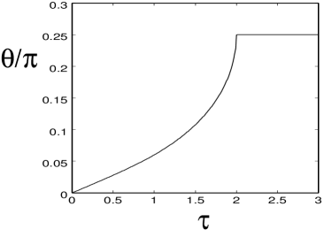
In order to discuss the evolution of the pairing state, we define an angle as

$$\theta=\tan^{-1}\frac{a}{b}.$$ (41)

This angle $\theta$ characterizes the pairing state. For the case of $\theta=0$, we have the p-wave pairing state that corresponds to the $(3,3,1)$ state. Meanwhile, for the case of $\theta=\pi/4$, we have the Pfaffian state. In Fig.Β 3, we show the inter-layer tunneling dependence of $\theta$. Note that the Pfaffian state is stabilized in the $\tau>2$ region.

In Fig.Β 4, we show the inter-layer tunneling dependence of the gap $\Delta$. Note that there is a cusp at $\tau=2$. Reflecting the presence of the cusp in the gap, the ground state energy also has a cusp at $\tau=2$.

Now we discuss the possibility of the Haldane-Rezayi state, or d-wave pairing state. Since the $s$-wave pairing state is excluded as mentioned above, the next leading singlet pairing state is the d-wave pairing state. From the analysis of the gap equation, we find that for the d-wave pairing state $\Delta\sim 1.2$, which is smaller than that for the p-wave pairing state, in the region of $\tau<\tau_{c}$ where $\tau_{c}\sim 0.8$ and the d-wave pairing state is not stabilized in $\tau>\tau_{c}$. However, in the above analysis we have neglected the effect of the long-range Coulomb interaction. Since the effect of it is expected to be larger for the p-wave pairing state than for the d-wave pairing state, it might be possible that the d-wave pairing state becomes stable due to the effect of the long-range Coulomb interaction. In addition, impurites may affect the p-wave pairing state more than the d-wave pairing state.

V Conclusion

In this paper, we have discussed the region of the inter-layer separation where the p-wave pairing state is stabilized and the effect of the inter-layer tunneling at $\nu=1/2$. The Pfaffian state is stable above the critical tunneling strength and there is a cusp at the transition point between the Pfaffian state and the state continuously connected with the $(3,3,1)$ state.

ACKNOWLEDGMENTS

This work was supported in part by a Grant-in-Aid from the Ministry of Education, Culture, Sports, Science and Technology.

REFERENCES

  • [1] The Quantum Hall Effect, 2nd ed., edited by R. Prange and S. Girvin (Springer Verlag, New York, 1990)
  • [2] Perspectives in Quantum Hall Effects, edited by Sankar Das Sarma and Aron Pinczuk (John Wiley & Sons, New York, 1997).
  • [3] R. B. Laughlin, Phys. Rev. Lett. 50, 1395 (1983).
  • [4] F. D. M. Haldane, in Ref.Β [1].
  • [5] B. I. Halperin, Helv. Phys. Acta. 56, 75 (1983).
  • [6] D. Yoshioka, A. H. MacDonald and S. M. Girvin, Phys. Rev. B 39, 1932 (1989).
  • [7] T. L. Ho, Phys. Rev. Lett. 75, 1186 (1995).
  • [8] G. Moore and N. Read, Nucl. Phys. B 360, 362 (1991).
  • [9] B. I. Halperin, Surf. Sci. 305, 1 (1994).
  • [10] F. D. M. Haldane and E. H. Rezayi, Phys. Rev. Lett. 60, 956 (1988); ibid, 60, 1886 (1988).
  • [11] T. Morinari, Phys. Rev. B 59, 7320 (1999).
  • [12] S. Q. Murphy, J. P. Eisenstein, G. S. Boebinger, L. N. Pfeiffer and K. W. West, Phys. Rev. Lett. 72, 728 (1994).
  • [13] M. Greiter, X. G. Wen and F. Wilczek, Nucl. Phys. B 374, 567 (1992).
  • [14] T. Morinari, Phys. Rev. B 62, 15903 (2000).
Refer to caption
FIG. 1.: The two-body correlation energy $E_{C}^{(2)}(m,n)/N^{2}$ for $(m,n)=(4,0),(3,1)$, and $(2,2)$ in units of $e^{2}/\epsilon\ell_{B}$.
Refer to caption
FIG. 2.: The energy $E_{C}^{(2)}(m,n)/N^{2}$ for $(m,n)=(2,0)$, and $(1,1)$ in units of $e^{2}/\epsilon\ell_{B}$.
Refer to caption
FIG. 3.: The inter-layer tunneling dependence of $\theta$.
Refer to caption
FIG. 4.: The inter-layer tunneling dependence of the gap $\Delta$.