Intrasubband plasmons in weakly disordered array of quantum wires

Abstract

The paper deals with the theoretical investigation of plasmons in weakly disordered array of quantum wires, consisting of finite number of quantum wires, arranged at an equal distance from each other. The array of quantum wires is characterized by the fact that the density of electrons of one ”defect” quantum wire was different from that of other quantum wires. At the same time it is assumed that ”defect” quantum wire can be arranged at an arbitrary position in array. It is shown that the amount of plasmon modes in weakly disordered array of quantum wires is equal to the number of quantum wires in array. The existence of the local plasmon mode, whose properties differ from those of usual modes, is found. We point out that the local plasmon mode spectrum is slightly sensitive to the position of ”defect” quantum wire in the array. At the same time the spectrum of usual plasmon modes is shown to be very sensitive to the position of ”defect” quantum wire.

Collective charge-density excitations, or plasmons in quantum wires (QW) are the objects of great physicist’s interest. Earlier plasmons in QW were investigated both theoretically [1, 2, 3, 4, 5] and experimentally [6, 7, 8]. In that papers it was shown that plasmons in QW possess some new unusual dispersion properties. Firstly, the plasmon spectrum depends strongly on the width of QW. Secondly, 1D plasmons are free from the Landau damping [2, 5] in the whole range of wavevectors.

From the point of view of practical application so-called weakly disordered arrays of low-dimensional systems are the objects of interest. Recently the plasmons in weakly disordered superlattices, formed of an finite number of equally spaced two-dimensional electron systems (2DES), were theoretically investigated [9, 10, 11, 12]. The weakly disordered superlattice is characterized by the fact that all 2DES possess equal density of electrons except one (”defect”) 2DES, which density of electrons differs from that of other 2DES. It was found that the plasmon spectrum of such a superlattice contains the local plasmon mode, whose properties differ from those of other plasmon modes. Notice that practically all flux of electromagnetic energy of plasmons, which correspond to the local mode, are concentrated in the vicinity of ”defect” 2DES. At the same time paper [12] denoted the opportunity of using the plasmon spectrum particularities to determine the parameters of defects in superlattice.

This paper deals with the theoretical investigation of plasmons in weakly disordered array of QW, consisting of a finite number $M$ of QW, arranged at planes $z=ld$ ($l=0,...,M-1$ is the number of QW, $d$ is the distance between adjacent QW). We suppose that all QW possess equal 1D density of electrons $N$ except one ”defect” QW whose density of electrons is equal to $N_{\rm{d}}$. So, the density of electrons in $l$-th QW can be expressed as $N_{l}=(N_{\rm{d}}-N)\delta_{pl}+N$. Here $p$ is the number of ”defect” QW arranged at the plane $z=pd$, $\delta_{pl}$ is the Cronecker delta. QW are considered to be placed into the uniform dielectric medium with dielectric constant $\varepsilon$. We consider the movement of electrons to be free in $x$-direction and is considerably confined in directions $y$ and $z$. At the same time we suppose that the width of all QWs is equal to $a$ in $y$-direction and is equal to zero in $z$-direction. By other words, each QW can be represented as a square quantum well with infinite barriers at $y=-a/2$ and $y=a/2$ and zero thickness in $z$-direction. At the same time we take into account only the lowest subband in each QW. In that case the single-particle wave function for the electron can be written in the form:

$$\psi_{k_{x},l}(x,y,z)=|k_{x},l\rangle=e^{\rmi k_{x}x}\varphi(y)\left[\delta(z-ld)\right]^{1/2},$$ (1)

where $\varphi(y)=\displaystyle{\sqrt{\frac{2}{a}}\cos{\frac{\pi y}{a}}}$, $k_{x}$ is the one-dimensional wave vector, describing the motion in $x$-direction. In that case the single-particle energy can be represented by such an expression:

$$E_{k_{x},l}=E_{0}+\frac{\hbar^{2}k_{x}^{2}}{2m^{*}}.$$

Here $E_{0}$ is the energy of subband bottom (for simplicity we may put $E_{0}=0$), $m^{*}$ is the effective mass of the electron.

To obtain the collective excitations spectrum we start with a standard linear-response theory in an random phase approximation. To obtain the collective excitations spectrum we consider $\delta n(\bf{r})$ which is the deviation of the electron density from its equilibrium value. After using the standard linear-response theory and the random phase approximation, $\delta n(\bf{r})$ can be related to the perturbation as

$$\delta n(x,y,z)=\sum_{\alpha,\alpha^{\prime}}\frac{f_{\alpha^{\prime}}-f_{\alpha}}{E_{\alpha^{\prime}}-E_{\alpha}+\hbar\omega}V_{\alpha\alpha^{\prime}}\psi_{\alpha^{\prime}}^{*}\psi_{\alpha},$$ (2)

where $\alpha=(k_{x},l)$ is a composite index which is defined by (1) and $f_{\alpha}$ is the Fermi distribution function, $V_{\alpha,\alpha^{\prime}}=\langle\alpha|V|\alpha^{\prime}\rangle$ are the matrix elements of the perturbing potential $V=V^{ex}+V^{H}$, $V^{ex}$ and $V^{H}$ are the external and Hartree potentials, correspondingly.

For our system equation (2) can be rewritten in the form

$$\delta n(q_{x},y,z)=\sum_{l^{\prime}}\Pi^{l^{\prime}}V_{l^{\prime}}\phi^{2}(y)\delta(z-l^{\prime}d),$$ (3)

where $\displaystyle{\Pi^{l^{\prime}}=\frac{1}{\pi}\int_{-\infty}^{\infty}dk_{x}\frac{f_{k_{x}+q_{x},l^{\prime}}-f_{k_{x},l^{\prime}}}{E_{k_{x}+q_{x},l^{\prime}}-E_{k_{x},l^{\prime}}+\hbar\omega}}$ is the noninteracting 1D polarizability (”bare bubble”) function, $V_{l^{\prime}}\equiv\langle k_{x},l^{\prime}|V|k_{x}+q_{x},l^{\prime}\rangle$. At zero temperature function $\Pi^{l}$ can be written as

$$\Pi^{l}=\frac{m^{*}}{q_{x}\pi\hbar^{2}}\ln{\frac{\omega^{2}-\displaystyle{\left(\frac{\hbar q_{x}k^{l}_{F}}{m^{*}}-\frac{\hbar q_{x}^{2}}{2m^{*}}\right)^{2}}}{\omega^{2}-\displaystyle{\left(\frac{\hbar q_{x}k^{l}_{F}}{m^{*}}+\frac{\hbar q_{x}^{2}}{2m^{*}}\right)^{2}}}}.$$ (4)

Here $\displaystyle{k^{l}_{F}=\frac{\pi N_{l}}{2}}$ is the Fermi wavenumber in $l$-th QW. In the long-wavelength limit (where $q_{x}\to 0$) function $\Pi^{l}$ can be written as $\displaystyle{\Pi^{l}=\frac{N_{l}}{m^{*}}\frac{q_{x}^{2}}{\omega^{2}}}$.

Notice, that the Hartree potential can be expressed through the perturbation [2] as

$$V^{H}(\bf{r})=\int\rmd\textbf{r}^{\prime}\frac{\it{e^{2}}}{\varepsilon|\textbf{r}-\textbf{r}^{\prime}|}\delta{\it n}(\textbf{r}^{\prime}).$$ (5)

Using equations (3) and (5) we get such an expression for matrix element $V^{H}_{l}=\langle k_{x},l|V^{H}(x,y,z)|k_{x}+q_{x},l\rangle$:

$$V^{H}_{l}=\sum_{l^{\prime}}\Pi^{l^{\prime}}V_{l^{\prime}}U_{l,l^{\prime}},$$ (6)

where

$$U_{l,l^{\prime}}=\frac{8e^{2}}{\varepsilon a^{2}}\int_{-a/2}^{a/2}\rmd y^{\prime}\int_{-a/2}^{a/2}\rmd yK_{0}(q_{x}[(y-y^{\prime})^{2}+(l-l^{\prime})^{2}d^{2}]^{1/2})\cos^{2}{\left(\frac{\pi y}{a}\right)}\cos^{2}{\left(\frac{\pi y^{\prime}}{a}\right)},$$

$K_{0}(x)$ is the zeroth-order modified Bessel function of the second kind. Collective excitations of QW array exist when equation (6) has nonzero solution $V^{H}$ in the case where the external perturbation $V^{ex}=0$. Hence, the intersubband plasmon dispersion relation has the form

$$\det|\delta_{l,l^{\prime}}-\Pi^{l^{\prime}}U_{l,l^{\prime}}|=0.$$ (7)

It should be noticed that when $M=2$ the dispersion relation (7) coincides with the dispersion relation for plasmons in double-layer QW system, obtained in [2].

Figure 1 shows the intrasubband plasmon spectrum (solid lines) in weakly disordered array of QW in the case where $p=0$. The $y$-axis gives the dimensionless frequency $\omega/\omega_{0}$ ($\omega_{0}^{2}=2Ne^{2}/\varepsilon m^{*}a^{2}$ is the plasma frequency), and the $x$-axis gives the dimensionless wavevector $q_{x}a^{*}$ ($a^{*}=\varepsilon\hbar^{2}/m^{*}e^{2}$ is the effective Bohr radius). As the model of QW we use heterostructure GaAs with the effective mass of electrons $m^{*}=0,067m_{0}$ ($m_{0}$ is the mass of free electron) and with the dielectric constant $\varepsilon=12,7$.

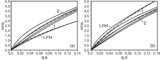
Figure 1: Dispersion curves of plasmons (solid curves) in weakly disordered array of QW with parameters $M=5$, $d=15a^{*}$, $a=20a^{*}$, $p=0$ for two values of the density of electrons of ”defect” QW: (a) $N_{\rm{d}}/N=0,5$, (b) $N_{\rm{d}}/N=1,5$. For comparison the dispersion curves for the plasmons in single QW with electron density $N_{\rm{d}}$ and $N$ are depicted by dashed curves 1 and 2, correspondingly.

As seen from figure 1, the intrasubband plasmon spectrum in finite array of QW contains $M$ modes. So, the number of modes in the spectrum is equal to the number of QW in the array. Notice, that with the increase of wavenumber $q_{x}$ the plasmon frequency $\omega$ also increases. At the same time the propagation of plasmons in weakly disordered array of QW is characterized by the presence of local plasmon mode (LPM). In the case where the density of electrons in ”defect” QW is less then the density of electrons in other QW ($N_{\rm{d}}<N$), the LPM lies in the lower-frequency region in comparison with the usual plasmon modes (figure 1a). Correspondingly, if $N_{\rm{d}}>N$, the LPM lies in the higher-frequency region in comparison with the usual ones (figure 1b). It should be emphasized that at the limit $q_{x}d\to\infty$, when the Coulomb interaction between electrons in adjacent layers is neglible, the LPM dispersion curve is close to the dispersion curve for the plasmons in single QW with the density of electrons $N_{\rm{d}}$. At the same time the dispersion curves for usual plasmon modes at the limit $q_{x}d\to\infty$ are gradually draw together and are close to the dispersion curve for plasmon in the single QW with the density of electrons $N$.

Now we consider the dependence of plasmon spectrum upon the value of 1D electron density in ”defect” QW. Figure 2 presents the dependence of plasmon frequency upon the ratio $N_{\rm{d}}/N$ in the case of fixed value of wavevector $q_{x}$ and for different positions of the ”defect” QW in the array. As seen from comparison of figure 2a,b,c the LPM spectrum depends weakly upon the position of ”defect” QW in array. However, the spectrum of usual plasmon modes is more sensitive to the position of ”defect” QW in the array. Notice, that the frequency of LPM increases when the value of ratio $N_{\rm{d}}/N$ is increased. At the same time the usual plasmon modes spectrum is characterized by such a features. As $p=0$ (figure 2a) when the value of ratio $N_{\rm{d}}/N$ is increased, the frequency of usual plasmon modes also increases. However when $p=1$ (figure 2b) the frequency of one of the usual plasmon modes (curve 2) does not practically depend upon the value of ratio $N_{\rm{d}}/N$. In the case where $p=2$ (figure 2c) there are already two plasmon modes (curves 1 and 3) which possess such a particularity.

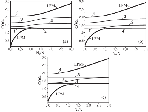
Figure 2: Dependence of plasmon frequency upon the ratio $N_{\rm{d}}/N$ when $q_{x}a^{*}=0,04$ and for three cases of ”defect” QW position in the array: (a) $p=0$, (b) $p=1$, (c) $p=2$.

In summary, we calculated the plasmon spectrum of finite weakly disordered array of QW, which contains one ”defect” QW. It is shown that amount of plasmon modes in the spectrum is equal to the amount of QW in array. It is found that the LPM, whose properties differ from those of other modes, exists in the plasmon spectrum. We point out that the LPM spectrum is slightly sensitive to the position of ”defect” QW in array. At the same time position of ”defect” QW exerts influence on the spectrum of usual plasmon modes. It is shown that under certain conditions the existence of plasmon modes, which spectrum does not depend upon density of electrons of ”defect” QW, is possible. Notice, that the above-mentioned features of plasmon spectra can be used for diagnostics of defects in QW structures.

References

References

- [1] Das Sarma S and Wu-yan Lai 1985 Phys. Rev. B 32 1401
- [2] Li Q P and Das Sarma S 1991 Phys. Rev. B 43 11768
- [3] Gold A and Ghazali A 1990 Phys. Rev. B 41 7626
- [4] Li Q P, Das Sarma S and Joynt R 1992 Phys. Rev. B 45 13713
- [5] Das Sarma S and Hwang E H 1996 Phys. Rev. B 54 1936
- [6] Hansen W, Horst M, Kotthaus J P, Merkt U, Sikorski Ch and Ploog K 1986 Phys. Rev. Lett. 58, 2586
- [7] Demel T, Heitmann D, Grambow P and Ploog K 1988 Phys. Rev. B 38 12732
- [8] Goñi A R, Pinczuk A, Weiner J S, Calleja J M, Dennis B S, Pfeiffer L N and West K W 1991 Phys. Rev. Lett. 67 3298
- [9] Gvozdikov V M 1990 Sov. J. Low Temp. Phys. 16 668
- [10] Jain J K and Das Sarma S 1987 Phys. Rev. B 35 928
- [11] Sy H K and Chua T S 1993 Phys. Status Solidi 176 131
- [12] Beletskii N N and Bludov Y V 1999 Radiofizika i Elektronika 4 93 (in Russian)