A case study of stratus cloud base height multifractal fluctuations

Abstract

The complex structure of a typical stratus cloud base height (or profile) time series is analyzed with respect to the variability of its fluctuations and their correlations at all experimentally observed temporal scales. Due to the underlying processes that create these time series, they are expected to have multiscaling properties. For obtaining reliable measures of these scaling properties, different methods of statistical analysis are used herein : power spectral density, detrended fluctuation analysis, and multifractal analysis. This broad set of diagnostic techniques is applied to a typical stratus cloud base height (CBH) data set; data were obtained from the Southern Great Plains site of the Atmospheric Radiation Measurement Program of the Department of Energy from a Belfort Laser Ceilometer. First, we demonstrate that this CBH time series is a nonstationary signal with stationary increments. Further, two scaling regimes are found, although the characteristic laws are quite similar ones. Next, the multi-affine scaling properties are confirmed. The scaling properties of the cloud base height profile of such a continental stratus are found to be similar to those of the marine cloud base height profiles studied by us previously. Some physical interpretation in terms of anomalous diffusion (or fractional random walk) is given for the continental case.

Keywords : stratus cloud, cloud base height, fluctuations, correlations, power spectrum, detrended fluctuation analysis, multifractals

I Introduction

The state of the atmosphere is governed by the classical laws of fluid motion and exhibits a great deal of correlation at various spatial and temporal scales. Knowing these space- and time-scale-dependent correlations is crucial, for example, in order to understand the short and long term trends in climate. In particular, clouds play an important role in the atmospheric energy budget. In order to model and predict climate successfully, we must be able to both describe the effects of clouds in the current climate and predict the complex chain of events that might modify the distributions and properties of clouds in an altered climate. Moreover, in order to improve the parameterization of clouds in climate models, it is important to understand the cloud properties and their changes within the cloud.

Modeling the impact of clouds is difficult because of their complex shapes, spatial distributions and varying particle size distributions and because of their differing effects on weather and climate. Clouds can reflect incoming sunlight, and so contribute to cooling, but they also absorb infrared radiation leaving the earth, and so contribute to warming. High cirrus clouds, for example, may have a nonnegligible impact on atmospheric warming. Low-lying stratus clouds, which are frequently found over oceans, can contribute to warming as well.[1]

A variety of physical processes takes place in the atmospheric boundary layer. At time scales of less than one day, significant fluxes of heat, water vapor and momentum occur due to entrainment, radiative transfer, and/or turbulence.[1, 2] The turbulent character of the motion in the atmospheric boundary layer (ABL) is one of its most important features. The turbulence[3] can be caused by a variety of processes, among them thermal convection and mechanical generation by wind shear.[2, 4, 5] This complexity of physical processes and interactions between them creates a variety of atmospheric responses. In particular, in a cloudy ABL, the radiative fluxes produce local sources of heating or cooling within the mixed layer and therefore can greatly influence its turbulent structure and dynamics. Moreover, variations in the turbulent structure and dynamics of the clouds cause subsequent changes in the cloud boundaries, especially in the height of cloud base. These variations lead to a complex structure for the cloud base height data (time) series. To analyze different aspects of the variability of its fluctuations and correlations at all experimentally observed temporal and spatial scales, one needs to apply a variety of diverse techniques of statistical analysis to the retrieved time series data. In what follows, we briefly present a few of these methods: a traditional technique - power spectral density, and rather new techniques, like a detrended fluctuation analysis, and multifractal analysis and then apply them to cloud base height data.

II Scaling

A Power spectral density

The power spectral density $S(f)$ of a signal $y(t)$ is obtained as a Fourier transform (FT) of the signal.[6, 7] The power spectrum provides information on the amplitude of the predominant frequencies present in the time series. This information allows one to identify periodic, multi-periodic, quasiperiodic or nonperiodic signals. Usually the logarithmic power spectrum plot is used to better distinguish between the broadband and periodic components. If the periods present are not of primary interest, then it is also used to evaluate the overall behavior of the time series. A power law dependence, and thus a linear dependence on a log-log plot, of $S(f)$ given by

$$S(f)~{}\sim~{}f^{-\beta}$$ (1)

that follows from the squared amplitude of the Fourier transform of the signal

$$S(f)=\lim_{T\longrightarrow\infty}\frac{1}{T}\left|\int_{-T}^{T}~{}e^{2\pi ift}~{}y(t)dt\right|^{2},$$ (2)

is a hallmark of a self-affine phenomenon that is underlying the data. The properties of the signal can be further classified as persistent or anti-persistent fluctuations, depending on the values of the spectral exponent $\beta$ in Eq. (1). If the signal possesses a tendency for repeating the sign of its fluctuations and, therefore, being of persistent type, then $2<\beta<3$; when fluctuations having opposite signs follow one another, i.e. when $1<\beta<2$, the signal is said to be anti-persistent.[7, 8] A signal with a spectral exponent obeying $1<\beta<3$ is a nonstationary signal with stationary increments. In this case, the time series created by the increments of a nonstationary signal has a spectral exponent $\beta$ within the interval [-1,1], and so is a stationary signal.[8] The latter property facilitates application of techniques of analysis to the increment signal. However the FT method, which produces second-order statistics, is insufficient to describe in full the signal scaling properties, because higher order moments may not be negligible. Strictly speaking, power spectrum analysis is suitable only for stationary time series. For more information on spectral time series analysis see [[9, 10, 11]]. Note that spectral analysis provides information on the scaling properties of the signal at high-frequency/short-time-scales, in contrast to the detrended fluctuation analysis method, which is reviewed next.

B DFA method and time dependence of the correlations

A method that relaxes the requirement of stationarity of the investigated signal is the detrended fluctuation analysis (DFA) method.[12] The DFA method is a tool used for sorting out long range correlations in a nonstationary self-affine time series with stationary increments.[13, 14, 15] The method has been used previously in the meteorological field. [16, 17, 18] It provides a simple quantitative parameter - the scaling exponent $\alpha$, which is a signature of the correlation properties of the signal. Let the signal $y(t)$ be defined between the beginning $t_{0}$ and end of the observations $t_{M}$, i.e. in $[t_{0},t_{M}]$. The DFA technique consists in dividing a time series $y(t)$ of length $N$ into an integer number $N/\mu$ of nonoverlapping boxes (called also windows), each containing $\mu$ points [12, 18] ($\mu$ = 4,5, …, ). The local trend $z(n)$ in each box is defined to be the ordinate of a linear least-squares fit of the data points in that box. The detrended fluctuation function $F^{2}(\mu)$ is then calculated using:

$$F^{2}(\mu)={1\over\mu}{\sum_{n=k\mu+1}^{(k+1)\mu}{\left[y(n)-z(n)\right]}^{2}}\qquad\mbox{for}\qquad k=0,1,2,\dots,\left(\frac{N}{\mu}-1\right).$$ (3)

Averaging $F^{2}(\mu)$ over the $N/\mu$ intervals gives the mean-square fluctuations that are assumed to follow a power law

$$<F^{2}(\mu)>^{1/2}\sim\mu^{\alpha}.$$ (4)

The DFA exponent $\alpha$ so obtained represents the correlation properties of the signal: $\alpha=1/2$ indicates that the changes in the values of a time series are random and, therefore, uncorrelated with each other, as in a Brownian random walk sequence. If $\alpha<1/2$ then the signal is anti-persistent (anti-correlated), and $\alpha>1/2$ indicate positive persistency (correlation) in the signal. It has been shown by Heneghan and McDarby[19] that the relationship $\beta=1+2\alpha$ holds true for stochastic processes, i.e. for fractional Brownian walks.

The $\alpha$-exponent value that holds true for a certain time interval called the scaling range, is a characteristic of the correlations in the fluctuations of a signal $y(t)$. It is of interest, however, to test whether the correlations maintain the same properties in shorter intervals within $[t_{0},t_{M}]$ or whether they change with time, as it should be anticipated for nonstationary time series data. In order to probe the existence of so-called locally correlated and decorrelated sequences,[13] one can construct an “observation box” with a certain width, $\nu$, place the box at the beginning of the data, calculate $\alpha$ for the data in that box, move the box by $\Delta\nu$ toward the right along the signal sequence, calculate $\alpha$ in that box, and so on through the $N$th point of the available data. Each $\alpha$-value is assigned to the end point of the box because all points in the box are needed in order to obtain $\alpha$. A time-dependent $\alpha$ may be expected for $t$ ranging from $\nu$ to $N$. This approach is suitable for cloud base height data because it can be expected to reveal changes in the correlation dynamics of the clouds at various times for a given time lag $\nu$. If such a time dependence is found, then a multifractal approach is to be suggested.[20, 21] In fact, it is expected that the usual fractal dimension[7] $D$ measuring the roughness of a signal[22] is directly related to $\alpha$ through[9, 22] $D=2-\alpha$, whence $D$ is time-dependent as well.

C Multifractal aspects

The scaling behavior of a signal $y(t)$ can change in a nonlinear fashion with the statistical moments, i.e. can be characterized by different scaling exponents. Such a signal is multi-affine and can be described through multifractal measures.[23, 24, 25, 26, 27] One approach which we will follow here consists in studying the intermittency and the roughness[24] of the signal. The intermittency is quantified adopting the singular measure analysis The first step that this technique requires is to define a basic measure $\varepsilon(1;l)$ as

$$\varepsilon(1;l)=\frac{|\Delta y(1;l)|}{<\Delta y(1;l)>},\qquad l=0,1,\dots,N-1$$ (5)

where $\Delta y(1;l)=y(t_{i+1})-y(t_{i})$ is the small-scale gradient field and $<>$ denotes an average over the $N$ data points

$$<\Delta y(1;l)>=\frac{1}{N}\sum_{l=0}^{N-1}|\Delta y(1;l)|.$$ (6)

Next we define a series of ever more coarse-grained and ever shorter fields $\varepsilon(r;l)$ where $0<l<N-r$ and $r=1,2,4,8\dots$. Thus the average measure in the interval $[l;l+r]$ is

$$\varepsilon(r;l)=\frac{1}{r}\sum_{l^{\prime}=l}^{l+r-1}\varepsilon(1;l^{\prime}).$$ (7)

The scaling properties of the generating function are then obtained for through the equation

$$<\varepsilon(r;l)^{q}>\sim\left(\frac{r}{N}\right)^{-K(q)},\quad q\geq 0.$$ (8)

Using $K(q)$-functions one can define[23] the generalized multifractal dimension[29, 30]

$$D(q)=1-\frac{K(q)}{q-1}.$$ (9)

Note that at $q=1$ the l’Hospital rule is used to obtain D(1).

Further, the multi-affine properties of a time-dependent signal $y(t)$ can also be described by the so-called $q$th order structure functions[23]

$$\left<|y(t_{i+r})-y(t_{i})|^{q}\right>\sim\tau^{qH(q)},\qquad i=1,2,\dots,N-r$$ (10)

with $\tau\equiv\Delta_{r}=t_{i+r}-t_{i}$. Whence $H(q)$ and $K(q)$ describe the multifractal scaling properties of nonlinear dynamic processes. In a monofractal case, $H(q)$ and and $K(q)$ take constant values.

D Hierarchy of exponents $h(\gamma)$

The multi-affinity of $y(t)$ means that one should use different scaling exponents $H(q)$ in order to rescale a signal in various scaling ranges. In other words, this also implies that local scaling exponent $\gamma$ exists[20] in order to characterize the local singularity of the signal. The density of points $N_{\gamma}(\Delta)$ that have the same local scaling exponent is usually assumed[31] to scale over the time span $\Delta$ (for any $r$) as

$$N_{\gamma}(\Delta)\sim\Delta^{-h(\gamma)}.$$ (11)

From Ref. [[32]] the following relations are found:

$$\gamma(q)=\frac{d(qH(q))}{dq}$$ (12)

$$h(\gamma(q))=1+q\gamma(q)-qH(q)$$ (13)

The $h(\gamma(q))$ function[20] is as naturally adapted to describe multi-affine signals as the multifractal spectrum for multifractal objects.[31]

Several of the methods reviewed in this section have been recently used in the meteorological field.[16, 17, 18, 23, 26, 33, 34, 35, 36]

III Data and data analysis

Next we apply the above methods to study the nonstationarity of cloud base height (CBH) data sets and the correlations in their fluctuations on all measured time scales; data are obtained at the Southern Great Plains site of the Atmospheric Radiation Measurement Program of the Department of Energy using a Belfort Laser Ceilometer (BLC) Model 7013C.[37] The ceilometer is a self-contained, ground-based, optical, active, remote sensing instrument with the ability to detect and process several cloud-related parameters, among them cloud base height, cloud extinction coefficient and cloud layer depth. The ceilometer system detects clouds by transmitting pulses of infrared light vertically into the atmosphere and analyzing the returned signals backscattered by the atmosphere. The receiver telescope detects scattered light from clouds and precipitation.[38] The ceilometer actively collects backscattered photons for about 5 seconds within every 30-second measurement period. The BLC measures the base height of the lowest cloud detected between 15 and 7350 m directly above mean ground level.

The cloud base height signal measured on Sept. 23-25, 1997 is plotted in Fig.1. Data consists of $N=7251$ data points, as for the purpose of this analysis we consider the record from 5:15 UTC on Sept. 23, through 17:40 UTC on Sept. 25, 1997. It is well representative of similar events often occurring on a shorter time interval.

The probability density function (PDF) for the cloud base height signal (data in Fig.1) is shown in Fig.2. The values of the abscissa, $\Delta y=y(t+\Delta t)-y(t)$ are unnormalized and therefore, given in meters. The cases $\Delta t=30$ s and $\Delta t=30$ min are displayed in Fig.2. They correspond to short and long time lags. Both PDFs are strongly non-Gaussian. The double pyramid triangular shape with a width growing with increased time lag is similar to that found in other meteorological cases.[39, 40]

We first check the stationarity of the data by applying a power spectral analysis. The power spectral density of the cloud base height data set is shown in Fig. 3. The upper curve represents the spectral density that is smoothed by applying a moving average over equidistant intervals on the log-scale. This procedure is anticipated to be better suited to identifying scaling properties of the spectrum.[6] It should be noted that the procedure may lead to a slight change in the slope of the linear fit that may to alter the scaling exponent slightly, as seen here from $\beta=1.46\pm 0.08$ to $\beta=1.33\pm 0.06$ for frequencies lower than 1/15 min^-1, i.e. $\sim$ 10^-3 Hz. Nevertheless, because $1<\beta<3$, we can conclude that, the cloud base height data are nonstationary with stationary increments. Futhermore, because $1<\beta<2$, the signal is anti-persistent. Note that the non-smoothed spectrum is more suitable for detecting characteristic frequencies and periods in the raw signal. The error bars in this paper are calculated according to standard techniques.[41]

Similar values for the spectral exponent, e.g. $\beta$=1.28$\pm$0.1 and $\beta$=1.49$\pm$0.08, are obtained in Ref. [[39, 40]] for cloud base height data measurements during the Atmospheric Stratocumulus Transition Experiment (ASTEX). ASTEX was designed to clarify the transition from stratocumulus to trade cumulus clouds[2] in the marine boundary layer in the region of the Azores Islands.[42] Studies of more cases are needed to clarify whether the slight difference in the scaling exponents between stratus over land, which is the subject of this paper, and stratocumulus clouds over ocean is physically and statistically significant or not.

The DFA leads to an $\alpha$ exponent equal to $0.18\pm 0.002$ for time lags less than 55 min, followed by an exponent $0.13\pm 0.001$, as indicated in the inset of Fig.4. Notice that the Heneghan and McDarby[19] relationship $\beta=1+2\alpha$ holds well for the shorter time lag region. Incidently we stress that two spectral regimes are hardly seen from the above spectral power density graph in Fig.3.

The time dependence of the correlations is next discussed. Results are plotted in Fig. 4 as a function of the cloud life time for $\nu=7$ h and $\Delta\nu=30$ min. The $\nu$ value is chosen such that the finite-size effects are avoided, while the $\Delta\nu$ value is somewhat arbitrarily chosen for an adequate display. Smaller values of $\Delta\nu$ lead to rougher curves representing the time-dependence of $\alpha$, nevertheless without significantly altering the overall results.

The generalized fractal dimensions $D(q)$ are shown in Fig. 5 and seen to decrease with $q$. The multi-affinity of the CBH signal is also observed from the nonlinearity of the functions $qH(q)$, $\gamma(q)$ and $K(q)$ in Figs.5 and 6. The value of the $H(q)$-function at $q=1$ defines the nonstationarity parameter $H_{1}$ that is a measure of the roughness of the signal, while $C_{1}$ at $q=1$

$$C_{1}=\left.\frac{dK(q)}{dq}\right|_{q=1}$$ (14)

usually defines the degree of intermittency of the signal.[23, 20, 24, 25]

The value obtained for the $H(q)$-function at $q=1$, $H(q=1)=H_{1}=0.21\pm 0.02$ is close to the $\alpha$-exponent of DFA method, $\alpha=0.18\pm 0.002$ of this study and is similar to the results for the cloud base height data measured during ASTEX, for which[39] $\alpha=0.24\pm 0.002$ for June 18, 1992 and $\alpha=0.21\pm 0.005$ for June 15, 1992 and for which[40] $H(q=1)=H_{1}=0.23\pm 0.04$ for June 14, 1992 and $H(q=1)=H_{1}=0.21\pm 0.03$ for June 15, 1992. If the cloud base height data series was a strictly defined monofractal signal, then one can expect that $\alpha=H_{1}$.[7]

Note that $q=1$ is a special case that corresponds to a monofractal behavior. Using l’Hospital’s rule in Eq. (14) one can obtain the information dimension of the CBH signal, if it scales as a monofractal

$$D(1)=1-\left.\frac{dK(q)}{dq}\right|_{q=1}$$ (15)

The dashed line in Fig. 5 defines the monofractal case $D(1)=1-C_{1}=0.90$. Having in mind that $C_{1}$ is related to the mean of $\varepsilon(r;l)$ for a one-dimensional field, we note that the singularities that contribute most to the $<\varepsilon(r;l)>$ occur on a set with fractal dimension $D(1)$. In order to compensate statistically for their sparse spatial distribution, in sharp contrast to a Gaussian process, these extreme events are far more rare but far more intense. There is no intermittency at all if $D(q)\equiv 1$, i.e. $C_{1}=0$.

The multi-affine properties of the signal are represented by the $h(\gamma)$ functions following Eq. (13) in Fig.7. Although the $h(\gamma)$-curve does not reach unity, it tends to some maximum value that corresponds to $\gamma_{0}\sim 0.21$, a value equal to the $\alpha$ exponent of the signal (Fig. 4). The crossing of the $x$-axis by the $h(\gamma)$-curve defines the minimum value $\gamma_{min}\sim 0$ that is related to the minimum value of the $\alpha$ exponent that is contained in the signal.[20] Here the value of $h(0)=0.70$, in agreement with the value 1-$qH(q)$ at its maximum as obtained from Fig.6, (see Eqs. (12) and (13)).

IV Conclusions

It is often asked what the numerical values of such above exponents mean, and whether they have any physical interpretation at all. Let us recall that the fractal dimension of a profile is a measure of its roughness, while generalized fractal dimensions have been given some thermodynamic interpretation elsewhere[43, 44] and here above (Sect.2). The above $\alpha$ exponent indicates that the cloud bottom is quite rough. The occurrence of two scaling regimes might be understood either from a mathematical point of view or a physical one. In the former case, Hu et al.[15] have indicated that such an occurrence can be due to different noises and different trends. On the other hand, the presence of two scaling regimes well separated by a crossover time lag may indicate that two processes occur in stabilizing, or not, the cloud base height data set (or profile). Indeed we had observed that the $\alpha$-exponent tends toward low values when the cloud is in quasi-equilibrium and reaches a high value when the cloud breaks apart[16]. We may conjecture here that the two scaling exponents describe two regimes of long time span (slow) correlations, which maintain stable droplets, and one at shorter time scales for fast correlations between droplets for both agglomeration or cloud fracture process. More cases need to be studied, however, in order to provide a more precise interpretation of these so close values of the $\alpha$-exponents.

Let us also recall that the simplest interpretation of a stochastic signal is through the notion of (fractional or not) Brownian motion, or random walk. In so doing, one can interpret the CBH signal as mimicking the distance from the origin (the initial time) traveled by a particle diffusing, e.g. on a lattice. An anomalous diffusion occurs if the signal correlations are not strictly characterized by the laws governing classical Brownian motion, but by other types of power laws.[45, 46] If those power laws are characterized by time-dependent exponents, then multifractality is expected. Usually the fractal dimension of a strange attractor measures the minimum number of components of the phase space necessary to describe the dynamic process. No such fractal dimension has been studied here. It would be interesting to look for it in order to define how many interrelated physical parameters are necessary to describe the CBH variability, i.e. pressure, temperature, humidity, wind velocity, etc. Following that line of thought, we can consider the CBH as representing stochastically driven turbulent eddies, in which phase transitions occur in three-dimensional space. In so doing the CBH is exactly a visual observation of these transitions in eddies moving up and down and horizontally in a stochastic way, as a random walk. In our case, the data set being studied is not really representing a particle in a 3D space but rather a projection on a 1D space; only the bottom of the cloud, projected on a vertical axis is studied with respect to its up and down motion, - just like particle undergoing (fractional or not) Brownian motion in a plane.

In summary, after recalling a few statistical analysis techniques, we have applied them to a typical continental stratus cloud base height profile data set. We have demonstrated that the CBH profile is a nonstationary anti-persistent signal with stationary increments. The spectral exponent found has a value similar to the one for stratoculumus clouds over the ocean reported by some of us in another study. The multi-affine scaling properties of the data series found reflect the complexity of the processes that produce them. Further work should be directed toward relating the scaling properties expressed through these statistical parameters to the dynamical properties of the clouds, an important step toward understanding, modeling and predicting their dynamical behavior.

V Acknowledgments

This research was partially supported by Battelle grant number 327421-A-N4. We acknowledge collaboration of the U.S. Department of Energy as part of the Atmospheric Radiation Measurement Program. MA thanks A. Pȩkalski for comments.

Figure Captions

Figure 1 – Cloud base height signal measured on Sept. 23-25, 1997 at the Southern Great Plains site of the Atmospheric Radiation Measurement Program of the Department of Energy. The abscissa marks the time in hours after 0 UTC on Sept. 23, 1997. The data series contains 7251 data points.

Figure 2 – Probability density function $P(\Delta y,\Delta t)$ (PDF) of the cloud base height signal measured on Sept. 23-25, 1997 (data in Fig. 1). The values on the abscissa, $\Delta y$, are given in meters. Triangles correspond to short time lag $\Delta t=30$ s equal to the discretization step of the data series, and circles mark the long time lag PDF with $\Delta t=30$ min. None of the PDF curves is displaced.

Figure 3 – Power spectrum $S(f)$ of the cloud base height signal measured on Sept. 23-25, 1997. The upper curve represents the smoothed spectra, vertically displaced by two decades, that scales with a spectral exponent $\beta=1.33\pm 0.06$.

Figure 4 – The local $\alpha$-exponent (black circles) given by the Detrended Fluctuation Analysis method as a function of time for the cloud base height (CBH) data measured on Sept. 23-25, 1997. Error bars are indicated. The rescaled (divided by a factor 3000) CBH signal is shown by dots. Inset: Log-log plot of the DFA-function Eq.(4), showing the scaling exponents $\alpha_{1}=0.18$, $\alpha_{2}=0.13$, and the crossover time lag at 55 min.

Figure 5 – Hierarchy of generalized dimensions $D(q)$ for the CBH data in Fig.1. The straight line is drawn to enhance the value $q_{s}$ at which the $D(q)$ function starts to deviate from a linear dependence. The dashed line defines the monofractal case $D(1)=0.90$; from Eq.(14) one thus finds $C_{1}$=0.10. The $K(q)$-function defined through Eq. (8) indicates the intermittency of the signal.

Figure 6 – The hierarchy of exponents $qH(q)$ and $\gamma(q)$ indicating the multi-affine properties of the continental stratus cloud base height (CBH) data measured on Sept. 23-25, 1997. For $q=1$, $H_{1}=0.21\pm 0.02$ is a parameter of nonstationarity.

Figure 7 – The $h(\gamma)$-curve for the stratus continental cloud base height data measured on Sept. 23-25, 1997; data in Fig. 1.

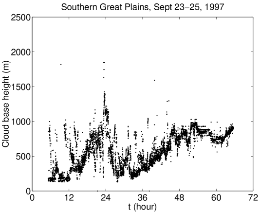
FIG. 1.: Cloud base height signal measured on Sept. 23-25, 1997 at the Southern Great Plains site of the Atmospheric Radiation Measurement Program of the Department of Energy. The abscissa marks the time in hours after 0 UTC on Sept. 23, 1997. The data series contains 7251 data points.

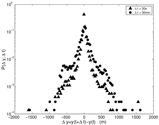
FIG. 2.: Probability density function $P(\Delta y,\Delta t)$ (PDF) of the cloud base height signal measured on Sept. 23-25, 1997 (data in Fig. 1). The values on the abscissa, $\Delta y$, are given in meters. Triangles correspond to short time lag $\Delta t=30$ s equal to the discretization step of the data series, and circles mark the long time lag PDF with $\Delta t=30$ min. None of the PDF curves is displaced.

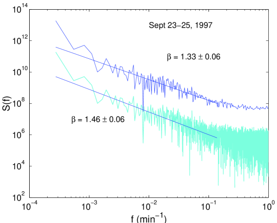
FIG. 3.: Power spectrum $S(f)$ of the cloud base height signal measured on Sept. 23-25, 1997. The upper curve represents the smoothed spectra, vertically displaced by two decades, that scales with a spectral exponent $\beta=1.33\pm 0.06$.

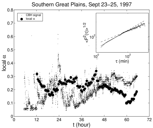
FIG. 4.: The local $\alpha$-exponent (black circles) given by the Detrended Fluctuation Analysis method as a function of time for the cloud base height (CBH) data measured on Sept. 23-25, 1997. Error bars are indicated. The rescaled (divided by a factor 3000) CBH signal is shown by dots. Inset: Log-log plot of the DFA-function Eq.(4), showing the scaling exponents $\alpha_{1}=0.18$, $\alpha_{2}=0.13$, and the crossover time lag at 55 min.

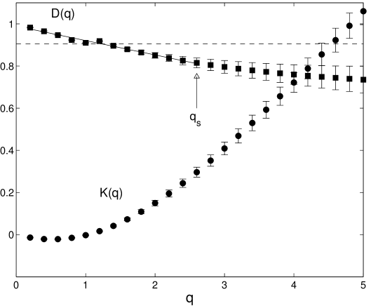
FIG. 5.: Hierarchy of generalized dimensions $D(q)$ for the CBH data in Fig.1. The straight line is drawn to enhance the value $q_{s}$ at which the $D(q)$ function starts to deviate from a linear dependence. The dashed line defines the monofractal case $D(1)=0.90$; from Eq.(14) one thus finds $C_{1}$=0.10. The $K(q)$-function defined through Eq. (8) indicates the intermittency of the signal.

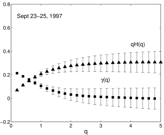
FIG. 6.: The hierarchy of exponents $qH(q)$ and $\gamma(q)$ indicating the multi-affine properties of the continental stratus cloud base height (CBH) data measured on Sept. 23-25, 1997. For $q=1$, $H_{1}=0.21\pm 0.02$ is a parameter of nonstationarity.

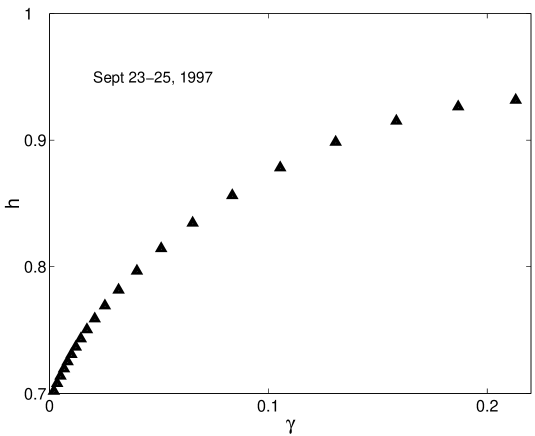
FIG. 7.: The $h(\gamma)$-curve for cloud base height data measured on Sept. 23-25, 1997.

REFERENCES

- [1] D. G. Andrews, An Introduction to Atmospheric Physics (Cambridge University Press, Cambridge, 2000)
- [2] J. R. Garratt, The Atmospheric Boundary Layer (Cambridge University Press, Cambridge, 1992)
- [3] U. Frisch, Turbulence: The legacy of A.N. Kolmogorov (Cambridge University Press, Cambridge, 1995)
- [4] H.A. Panofsky and J.A. Dutton, Atmospheric Turbulence (John Wiley & Son Inc., New York, 1983)
- [5] A. G. Driedonks and P.G. Duynkerke, Bound. Layer Meteor. 46, 257 (1989)
- [6] T.W. Körner, Fourier Analysis (Cambridge Univ. Press, Cambridge, 1988)
- [7] K. J. Falconer, The Geometry of Fractal Sets (Cambridge Univ. Press, Cambridge, 1985)
- [8] D.L. Turcotte: Fractals and Chaos in Geology and Geophysics (Cambridge University Press, Cambridge 1997)
- [9] B.D. Malamud and D.L. Turcotte, J. Stat. Plann. Infer. 80, 173 (1999)
- [10] M.S. Taqqu, V. Teverovsky and W. Willinger, Fractals 3, 785 (1995)
- [11] P.J. Brockwell and R.A. Davis, Time Series : Theory and Methods (Springer-Verlag, Berlin,1991)
- [12] C.-K. Peng, S.V. Buldyrev, S. Havlin, M. Simmons, H.E. Stanley and A.L. Goldberger, Phys. Rev. E 49, 1685 (1994)
- [13] N. Vandewalle and M. Ausloos, Physica A 246, 454 (1997)
- [14] M. Ausloos and K. Ivanova, Int. J. Mod. Phys. C 12, 169 (2001)
- [15] K. Hu, Z. Chen, P.Ch. Ivanov, P. Carpena and H.E. Stanley, Phys. Rev E (in press) (2001)
- [16] K. Ivanova, M. Ausloos, E.E. Clothiaux and T.P. Ackerman, Europhys. Lett. 52, 40 (2000)
- [17] E. Koscielny-Bunde, A. Bunde, S. Havlin, H. E. Roman, Y. Goldreich and H.-J. Schellnhuber, Phys. Rev. Lett. 81, 729 (1998)
- [18] K. Ivanova and M. Ausloos, Physica A 274, 349 (1999)
- [19] C. Heneghan and G. McDarby, Phys. Rev E 62, 6103 (2000)
- [20] N. Vandewalle and M. Ausloos, Eur. Phys. J. B 4, 257 (1998)
- [21] A.-L. Barabasi and T. Vicsek, Phys. Rev. A 178, 2730 (1991)
- [22] M. Ausloos, in Computational Statistical Physics. From Billiards to Monte Carlo, K.H. Hoffmann and M. Schreiber, Eds. (Springer, Berlin, 2001) pp.153-168
- [23] A. Davis, A. Marshak, W. Wiscombe and R. Cahalan, J. Geophys. Res. 99, 8055 (1994)
- [24] N. Vandewalle and M. Ausloos,Int. J. Mod. Phys. C 9, 711 (1998)
- [25] K. Ivanova and M. Ausloos, Eur. Phys. J. B 8, 665 (1999); Err. 12, 613 (1999)
- [26] K. Ivanova and T. Ackerman, Phys. Rev. E 59, 2778 (1999)
- [27] E. Canessa, J. Phys. A 33, 3637 (2000)
- [28] P. Bergé, Y. Pomeau and Ch. Vidal, L’ordre dans le chaos (Hermann, Paris, 1984) ch. IX
- [29] P. Grassberger, Phys. Rev. Lett. 97, 227 (1983)
- [30] H.G.E. Hentschel and I. Procaccia, Physica D 8, 435 (1983)
- [31] T.C. Halsey, M.H. Jensen, L.P. Kadanoff, I. Procaccia and B.I. Shraiman, Phys. Rev. A 33, 1141 (1986)
- [32] A.-L. Barabasi, P. Szepfalusy and T. Vicsek, Physica A 178, 17 (1991)
- [33] A.A. Tsonis, P.J. Roeber and J.B. Elsner, Geophys. Res. Lett. 25, 2821 (1998)
- [34] A.A. Tsonis, P.J. Roeber and J.B. Elsner, J. Climate 12, 1534 (1999)
- [35] P. Talkner and R.O. Weber, Phys. Rev. E 62, 150 (2000)
- [36] K. Ivanova, E.E. Clothiaux, H.N. Shirer, T.P. Ackerman, J. Liljegren and M. Ausloos, J. Appl. Meteor. in press
- [37]
- [38]
- [39] N. Kitova, K. Ivanova, M. Ausloos, T.P. Ackerman and M. A. Mikhalev, Int. J. Modern Phys. C, in press
- [40] N. Gospodinova, K. Ivanova, E.E. Clothiaux and T. Ackerman, “Multifractal characterization of nonstationarity and intermittency of cloud base height signals,” In Proceedings of the 11th International School on Quantum Electronics: Laser physics and Applications, Varna, Bulgaria, Sept. 18-22, 2000.
- [41] A.C. Bajpai, I.M. Calus and J.A. Fairley, Statistical Methods for Engineers and Scientists (Wiley, Chichester, 1978)
- [42] P.G. Duynkerke, H.Q. Zhang and P.J. Jonker, J. Atm. Sci. 62, N16, 2763 (1995)
- [43] E. Domany, S. Alexander, D. Bensimon and L.P. Kadanoff, Phys. Rev. B 28, 3110 (1983)
- [44] L.P. Kadanoff, Statistical Physics (World Sc., Singapore, 2000)
- [45] J.-P. Bouchaud and A. Georges, Phys. Rep. 195, 127 (1990)
- [46] R. Metzler and J. Klafter, Phys. Rep. 339, 1 (2000)