[

Effect of dielectric responses on localization in 1D random periodic-on-average systems

Abstract

Dielectric response effects on wave localization in random periodic-on-average layered systems (POAS) are studied. Based on Monte Carlo simulations and products of Random Matrices, statistics of the Lyapunov exponent are determined efficiently for very long systems. A novel oscillatory behavior for Lyapunov exponent is found and explained for mildly strong scattering conditions. We also show the emergence of strongly localized states in metallic layered systems with intermediate disorder for frequencies above the plasma frequency $\omega_{p}$ of metals, as is not shown in dielectrics. Furthermore, the violation of universal single parameter scaling behaviors in different regimes of multiple scattering is discussed.

PACS numbers: 72.15.Rn, 03.65.Sq, 05.45.+b, 42.25.Bs

]

The realization that Anderson localization in electronic systems[1] is due to wave interference between scattered waves from random scatters has stimulated vivid research in search of wave localization in condensed matter physics[2, 3, 4, 5, 6]. Further progress have been made to the aspects of photon localization[7, 8, 9, 10, 11, 12, 13, 14, 15, 16, 17] because photons may open a new realm of optical and microwave phenomena, and provided an analogous insight into Anderson localization transition undisturbed by Coulomb interaction.

It had been shown individual scatter’s response to the wave fields influence wave localization properties remarkably in entirely random systems , such as the strong localization for acoustic waves in bubbly liquids[6]. The same issues should exist in POAS for the intricate interplay between order and disorder. One-dimensional systems are particular interesting as they provide insights to the problems of wave localization in general and are suitable for testing various ideas. Two qualitatively different regimes of localization are exhibited[11, 14]. For band gap states, single parameter scaling (SPS) with universal behaviors is observed; however, the scaling is restored only when the randomness of defects exceeds a certain threshold for the situation of weak dielectric mismatch between constituent layers[14].

The scope of the Communication is twofold. The main interest is to understand multiple scattering effects on wave localization and the SPS in 1D systems. Particular attentions are paid for mildly scattering conditions; that is, the dielectric mismatch between layers is not too large. The secondary interest lies in preliminary exploration of dispersive or absorptive media on wave localization. Here, we consider EM wave localization in 1D random superlattices made of two alternating layers, the so-called Kronig-Penny model. As usual, the wave transmission can be tackled in exact manner by the transfer-matrix method[14]. Nevertheless, the approach encounter the difficulty that transmission coefficient in that formulation falls bellow the computer round-off accuracy for very long systems[16]. For the practical purpose, we improve the Herbert-Jones-Thouless formula[19] widely known in the study of disordered electronic quantum systems to study electromagnetic wave localization, with electron energies being replaced by wave frequencies; consequently, universal behaviors for very long structures can be studied quantitatively. Numerically, the state of wave fields is formulated by a vector $v_{n}=(E_{n},E^{{}^{\prime}}_{n})^{t}$ with the electric field $E_{n}$, its spatial derivative $E^{{}^{\prime}}_{n}$, the wave number $k=\omega/c$ in vacuum, and the superscript $t$ represents the matrix transposition. The relation between the (n+1)th layer and the nth layer is specified by the transfer matrix ${\rm M_{n}}$:

$${\rm M}_{n}=\left(\begin{array}[]{clr}{\rm cos}(k_{n}d_{n})&\frac{1}{k_{n}}{\rm sin}(k_{n}d_{n})\\ -k_{n}{\rm sin}(k_{n}d_{n})&{\rm cos}(k_{n}d_{n})\end{array}\right)$$ (1)

where $k_{n}=k\sqrt{\epsilon_{n}(\omega)}$, and the n-th layer width $d_{n}$ . In dielectrics, the dielectric constant $\epsilon_{n}$ is real; however, in metals, the dielectric constant $\epsilon_{n}$ is complex and frequency-dependent. Lyapunov exponent(LE) and its variance (VAR), $\mbox{Var}(\lambda)=\langle\lambda^{2}\rangle-\langle\lambda\rangle^{2}$, are the transmission quantities considered here. The VAR represents the fluctuations for the LE in defect configurations. The LE can be computed as follows [19]:

$$\lambda={\rm Re}\lim_{N\rightarrow\infty}\frac{1}{L}\left\langle\ln\left({\rm Tr}\prod_{n=1}^{2N}{\rm M}_{n}({\rm Conj}(\epsilon_{n}))\right)\right\rangle$$ (2)

where $2N$ is the total number of alternating layers, $L$ is the average total length of considered systems, Tr is the trace operator, Conj means taking complex conjugate, and the symbol $\langle...\rangle$ means the ensemble average over the uniform distribution of random configurations. The complex conjugate of the dispersive dielectric function $\epsilon_{n}$ is taken for the reciprocity of the absorptive systems [16].

Consider 1D superlattices made of two alternating layers A and B with the dielectric response functions $\epsilon_{A}$ and $\epsilon_{B}$ respectively. Random configurations are introduced by varying the layer $B$ width $d_{B}$ uniformly in the interval $(\langle d_{B}\rangle(1-\sigma),\langle d_{B}\rangle(1+\sigma))$ , where $\sigma\in(0,1)$ represents the randomness while the width of $A$ layer $d_{A}$ is kept fixed. A series of Random Matrices ${\rm M}_{n}$ are generated to obtain the LE and VAR by the Monte Carlo simulation in Eq.(2). In practice, the accurate LE and VAR are attained by letting the total length of layered systems to be several thousand times larger than the decaying length-scale $\lambda^{-1}$ (the inverse of Lyapunov exponent), representing exactly the localization length in absorption free cases. Sufficient times of ensemble averages are thus determined by the evaluation of numerical stability with the length of the system.

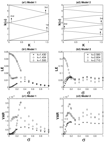
FIG. 1.: Model 1: (a1) Band structures where K is Bloch wave number in periodic layers and ${\rm k}=\omega/c$ is the wave number in free space. (b1) Lyapunov exponent vs. randomness $\sigma$. (c1) Variance vs. randomness $\sigma$. Model 2 : (a2) Band Structures. (b2) Lyapunov exponent vs. randomness $\sigma$. (c2) Variance vs. $\sigma$.

To begin with, multiple scattering effects on wave localization in dielectrics are studied. Two models are demonstrated. Model 1 is a weakly scattering model with the dielectric contrast $\epsilon_{B}/\epsilon_{A}=1.21$ while Model 2 is the mildly strong scattering model with the contrast $\epsilon_{B}/\epsilon_{A}=6.25$. The band structures of original periodic layers[18] for Model 1 and 2 are shown in Figs. 1 (a1) and (a2). The LE and VAR in Model 1 and 2 are compared in Figs. 1(b1 - c1) and (b2 - c2). The parameters, $\epsilon_{A}=1,d_{A}=\langle d_{B}\rangle=d=1$, are taken in computations. The symbols ‘$*$’,‘$\circ$’, and ‘$\diamond$’ denote states in bands, band edges, and gaps respectively hereafter.

In Model 1, previous results are reproduced[14]. In Fig. 1 (b1), the LE decreases monotonically with randomness in the first gap around $k=1.50$ since the established Bragg wave coherence has been gradually destroyed, the so-called enhanced transmission due to disorder[10]. In the allowed band $k=1.43$, the LE initially increases with the randomness and then decreases for large randomness. In the band edge $k=1.454$, the LE decreases first, then increase slightly, and finally decrease monotonically with the randomness $\sigma$. The behavior is due to the interplay between order and disorder in the systems. Moreover, the curves for these states merge for large disorder, the manifestation of universal single parameter scaling[14]. In Fig. 1 (c1), the plot of VAR vs. randomness $\sigma$ is demonstrated. The VAR at these frequencies shows similar behaviors. When the randomness of defects is large in the ensembles, the effect of self-averaging is effective because random fluctuations for these states are almost cancelled leading to the reduction in VAR. For nearly periodic configurations, the wave localization length in a gap regime is much smaller than the mean distance between defects so that the defects are isolated for incident waves. The increase of randomness can only cause minor growth of fluctuations due to the increase of the localization length. The competition between the two mechanisms results in the observed maximal VAR.

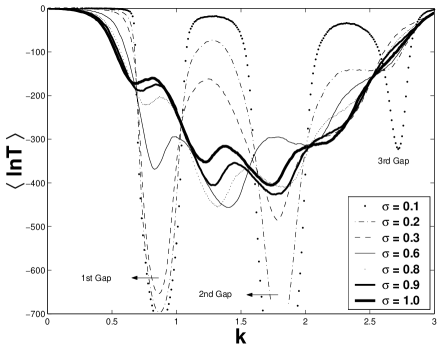
FIG. 2.: The average transmission $\langle{\rm lnT}\rangle=-2{\lambda}N$ vs. frequency ${\rm k}$ with different randomness $\sigma$.

In Model 2, mildly strong scattering case, novel oscillatory behaviors of the LE and VAR in the 3rd gap are exhibited above the randomness $\sigma=0.3$ in Figs. 1 (b2) and (c2), which is very different from the behaviors of Model 1 in Figs. 1 (b1) and (c1). To understand the disorder effects, we plot the average transmission spectrum ${\rm\langle lnT\rangle}$ covering the lowest three pass bands and gaps of Model 2 for the randomness $\sigma$ from $0.1$ to $1$, as is shown in Fig. 2. First, we observe well defined band structures, transmission enhancement in gaps, and inhibition in pass bands appears as usual when the minor randomness ranging from $\sigma=0.1$ to $\sigma=0.3$ is presented. With large randomness above $\sigma=0.3$, we observe the enormous overlap between original band structures emerges from the high frequency states from $k=2$ to $3$ and then extends to the states from $k=1$ to $3$. In addition, it is noticed that the oscillatory behavior only occurs for these states. Take the 2nd gap for example, the transmission initially enhance till the randomness $\sigma=0.6$, and then weaken for larger randomness. For the 3rd gap, the oscillation in the transmission corresponds to the oscillation in LE in Fig. 1 (b2). For the first gap and pass band where the overlap with other states is negligible, the behavior does not exist. Therefore, the novel oscillation in LE could be explained as a result of the overlap between band structures in these states for large randomness.

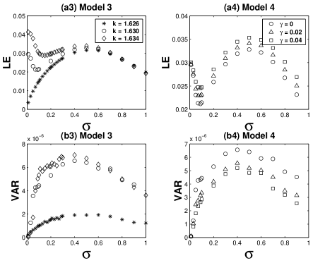
FIG. 3.: Model 3: (a3) Lyapunov exponent vs. randomness $\sigma$. (b3) Variance vs. randomness $\sigma$ . Model 4: (a4) Lyapunov exponent vs. randomness $\sigma$ at the frequency $k=1.630$ in Model 3. The circle $\rm o$, triangle $\triangle$, and square $\Box$ represent the cases with electron damping rates $\gamma$ = $0$, $0.02$, and $0.04$, respectively. (b4) Variance vs. randomness $\sigma$.

Turn to the secondary interest. As a preliminary inspection on dispersive media, the statistics of LE and VAR for metallic slabs are demonstrated in Fig. 3. The layers $B$ are composed of metals with the dielectric response function $\epsilon_{B}:$

$$\epsilon_{B}(\omega)=1-\frac{{\omega_{p}}^{2}}{\omega(\omega+i\gamma)}$$ (3)

where $\omega_{p}$ is the plasma frequency, $\omega$ the EM wave frequency, and $\gamma$ the electron damping rate which leads to residual wave energy dissipation. The fixed parameters for layer $A$ are the same as previous Model 1 and 2. The only difference is the introduction of the plasma frequency $\omega_{p}d/c=1$ ( $c$ : speed of light in vacuum) of metallic slabs, and the reduced wave number $k=\omega d/c=\omega/\omega_{p}$.

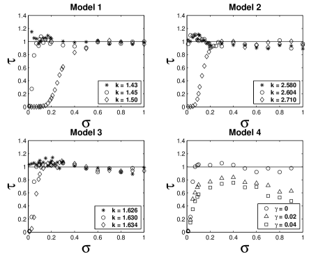
FIG. 4.: Scaling parameter $\tau$ vs. randomness for Model 1, Model 2, Model 3, and Model 4, respectively. The horizontal solid line denotes the universal value $\tau=1$.

We focus on frequencies above the plasma frequency $\omega_{p}$ since waves can only propagate above the plasma frequency. It is noted that the dielectric contrast $\epsilon_{B}/\epsilon_{A}$ in this case is real in the absence of residual absorption. The residual absorption can be turned off by taking electron damping rate $\gamma$ as zero. The frequencies in later computations are taken from the first gap above $\omega_{p}$. In Fig. 3 (a3), a peculiar feature not shown in dielectrics occurs. For the gap state $k=1.634$, the contrast between the LE at the randomness $\sigma\simeq 0$ and 0.5 is much smaller than Model 1 (See Fig. 1 (b1)). Moreover, the LE is even larger with the intermediate randomness $\sigma=0.5$ than the LE with the minor randomness $\sigma\simeq 0$ at the edge state $k=1.630$. The explanations are as follows. The dispersive response of metals makes the dielectric contrast between layers lower for higher frequencies, which leads to the reduction of extra transmission difference between the pass bands and gaps. So, the feature is attained by diminishing the difference of these states in LE in its dielectric counterpart at minor randomness $\sigma\simeq 0$ in qualitative agreement with the behavior in Fig. 3 (a3). The effect is remarkable with nearly periodic layers because individual layer’s responses can be accumulated by the Bragg wave coherence. This suggests versatile ways could be available in the fabrication of the EM wave devices operating near band edges in POAS with dispersions[20]. In Fig. 3 (b3), the VAR agrees qualitatively with Model 1 although the shape of the VAR is not so sharp as Model 1. In addition, the VAR does not merge for these frequencies at large degrees of disorder, the implication of the SPS violation to be discussed later. One may wonder the peculiar feature may be smeared out with residual absorption. To confirm the point, the LE vs. randomness figure is plotted in Fig. 3 (a4) as comparison. We see the feature can be strengthened further because the LE increases noticeably with the damping rate $\gamma$ for large randomness. The VAR decreases with the damping rate in Fig. 3 (b4), as is shown similarly in the reference[16] .

Single parameter scaling (SPS) is studied next to understand its dependence on constituent scatter properties, as is shown in Fig. 4. The SPS indicates that the LE is not an independent parameter and is related to its variance in a universal way [1, 15]:

$$\tau=\frac{\mbox{Var}(\lambda)}{\lambda}L=1,$$ (4)

where $L$ is the length of the system. The horizontal solid line represents the universal value $\tau=1$. In Fig. 4, for the weakly scattering case, the SPS is obeyed for all band gap states in Model 1. This is reasonable since weak gaps make the macroscopic wave coherence easily broken by disorders, as is shown by Deych et al[15]. However, the SPS is not rigorously met for large randomness with slight fluctuations in $\tau$ in Model 2 and Model 3. The phenomenon is universal in the two models, one is dielectric and the other is dispersive, even though their detailed LE and VAR disagree. In retrospection, in Model 3, the dispersive dielectric response in metals generates an intrinsically larger dielectric mismatch than Model 1. Therefore, the degree of deviations near the universal value $\tau=1$ can be recognized as the signature of the gradual dominance of multiple scattering effects. In Model 4, we show that the parameter $\tau$ decreases with electron damping rate as well as randomness. Moreover, the residual absorption makes the value of the parameter ${\tau}$ smaller than one. From above discussions, the SPS depends much on varied dielectric responses of constituents. In weak scattering cases, the SPS is met for allowed bands, gaps, and edges. In mildly scattering cases, the parameter shows deviated fluctuations near the universal value $\tau=1$. However, in residual absorption cases, the parameter $\tau$ falls below the universal value.

In addition, for strongly scattering conditions, the SPS is violated for two possibilities in our investigations. One is due to narrow band structures created in underlying periodic layers resulting in tremendous overlap between these bands in the presence of randomness[17]. The other possibility checked by us, however, is the generation of wide bands by exchanging the sequence of the same constituent layers such that the overlap does not emerge and gaps are robust enough to resist the addition of randomness. Therefore, to sum up, the band structures of underlying periodic layers in various scattering regimes determines the distinctive wave localization properties in POAS.

In conclusion, we have studied effects of dielectric response on wave localization and single parameter scaling behaviors in periodic-on-average systems. Novel oscillatory wave localization behaviors in the presence of mildly strong multiple scattering effects is found and explained numerically. For dispersive dielectric response, it is also shown that a strong localization occurs for intermediate degree of disorder in metallic layers, which was not found previously in dielectrics. The findings suggest the possible applications over optical devices operating near photonic band edges in dispersive periodic-on-average structures in parallel with photonic crystals[20]. Furthermore, the SPS is not rigorously met in the presence of multiple scattering effects or residual absorption in our studies.

The work was supported by National Center for Theoretical Sciences (Physics Division) in Hsinchu, Taiwan.

REFERENCES

- [1] P. W. Anderson, D. J. Thouless, E. Abrahams, and D. S. Fisher, Phys. Rev. B 22, 3519 (1980).
- [2] P. Sheng, B. White, Z. Q. Zhang, and G. Papanicolaou , Phys. Rev. B 34, 4757 (1986).
- [3] H. De Raedt, A. Lagendijk, and P. de Vries, Phys. Rev. Lett. 62, 47 (1989).
- [4] Norihiko Nishiguchi, Shin-ichiro Tamura, and Franco Nori, Phys. Rev. B 48, 2515 (1993).
- [5] M. M. Sigalas and C. M. Soukoulis, Phys. Rev. B 51, 2780 (1995)
- [6] Z. Ye and A. Alvarez, Phys. Rev. Lett. 80, 3503 (1998)
- [7] S. John, Phys. Rev. Lett. 58, 2486 (1987).
- [8] R. D. Meade, K. D. Brommer, A. M. Rappe, and J. D. Joannopoulos, Phys. Rev. B. 44, 13772 (1991).
- [9] E. Yablonovitch, T. J. Gmitter, R. D. Meade, A. M. Rappe, K. D. Brommer, and J. D. Joannopoulos, Phys. Rev. Lett. 67, 3380 (1991).
- [10] V. D. Freilikher, B. A. Liansky, I. V. Yurkevich, A. A. Maradudin, and A. R. McGurn, Phys. Rev. E. 51, 6301 (1995).
- [11] Y. A. Vlasov, M. A. Kaliteevski, and V. V. Nikolaev, Phys. Rev. B. 60, 1555 (1999).
- [12] M. Torres, F. R. M. D. Espinosa, D. Garcia-Pablos and N. Garcia, Phys. Rev. Lett. 82, 3054 (1999).
- [13] A. A. Chabanov, M. Stoytchev, and A. Z. Genack, Nature 404, 850 (2000).
- [14] L. I. Deych, D. Zaslavsky, and A. A. Lisyansky, Phys. Rev. Lett. 81, 5390 (1998).
- [15] Lev I. Deych, A. A. Lisyansky, and B. L. Altshuler, Phys. Rev. Lett. 84, 2678 (2000).
- [16] L. I. Deych, A. Yamilov, and A. A. Lisyansky, Phys. Rev. B. 64, 024201 (2001).
- [17] P. G. Luan and Z. Ye, Phys. Rev. E. 64, 066609 (2001).
- [18] where , is the Bloch wave number , is the wave number in the layer A, is the wave number in the layer B, and .
- [19] A. Crisanti, G. Paladin, and A. Vulpiani, Products of Random Matrices in Statistical Physics, (Springer-Verlag, Berlin, 1993).
- [20] T. Quang, M. Woldeyohannes, S. John, and G. S. Agarwal, Phys. Rev. Lett. 79 , 5238 (1997).