Electronic Properties of the Effective Singlet-Triplet Model

Abstract

In present work the effective singlet-triplet model for $CuO_{2}$-layer in the framework of multiband p-d model of strongly correlated electrons is obtained. The resulting Hamiltonian has a form of generalized singlet-triplet t-t’-J model for p-type superconductors and form of usual t-t’-J model for n-type superconductors. In the mean field approximation in X-operator representation we derived equations for Gorkov type Green functions. The symmetry classification of the superconducting order parameter in the case of tetragonal lattice resulted in $d_{x^{2}-y^{2}}$- and $d_{xy}$-types of singlet pairing for both p- and n-type superconductors while s-type singlet pairing don’t take place. Also normal paramagnetic phase of effective singlet-triplet model was investigated and the Fermi-type quasiparticle dispersion over Brillouin zone, density of states and evolution of Fermi level with doping were obtained.

1 Introduction

Almost twenty years passed from the discovery of High-$T_{c}$ Superconductivity (HTSC) but for now there is no widely accepted theory of pairing mechanism in cuprates of p- and n-type. The necessary ingredient for discussing possible mechanisms of HTSC is the band structure of the fermion-like quasiparticles. However, it is a difficult subject for ab initio calculations due to the strong electron correlations. For this reason we will use a model approach and in order to get an agreement with experimental data we will start with a realistic multiband p-d model of transition metal oxides.

The Hubbard model is often used to study electronic structure of strongly correlated electron systems (SCES). To take into account the chemistry of metal oxides the Hubbard model is generalized to the p-d model, a simplest version of such a model has been proposed by Emery [1] and Varma et al. [2]. In this 3-band p-d model only $d_{x^{2}-y^{2}}$ Cu and $p_{\sigma}$ O orbitals are considered. One of the important features omitted in this model is asymmetry of n-type (electrons doped) and p-type (holes doped) cuprates. Point is that the spin-exciton concerned with singlet-triplet excitation of two-hole term occurs only in p-type systems, but not in n-type [3]. Other feature is a non-zero occupancy of $d_{z^{2}}$ Cu orbitals [4]. There also a dependence between $T_{c}$ and occupancy of $d_{z^{2}}$ was found. Hence more realistic model of $CuO_{2}$-layer has to include $d_{x^{2}-y^{2}}$- and $d_{z^{2}}$- orbitals on copper and $p_{x}$-, $p_{y}$-, $p_{z}$- orbitals on oxygen as well. Such model is the multiband p-d model that has been proposed by Gaididei and Loktev [5]:

$$H_{p-d}=\sum_{r}H_{d}(r)+\sum_{i}H_{p}(i)+\sum_{<r,i>}H_{pd}(r,i)+\sum_{<i,j>}H_{pp}(i,j),$$ (1)

where

$$H_{d}(r)=\sum_{\lambda,\sigma}\left[\varepsilon_{\lambda}^{d}\,d_{\lambda r\sigma}^{+}\,d_{\lambda r\sigma}+\frac{U_{\lambda}^{d}}{2}n_{\lambda r}^{\sigma}n_{\lambda r}^{\bar{\sigma}}\right.$$

$$\hbox to0.0pt{\hss${}-{}$}\left.\sum_{\lambda^{\prime},\sigma^{\prime}}\left(J_{\lambda\lambda^{\prime}}^{dd}d_{\lambda r\sigma}^{+}d_{\lambda r\sigma^{\prime}}d_{\lambda^{\prime}r\sigma^{\prime}}^{+}d_{\lambda^{\prime}r\sigma}-\sum_{r^{\prime}}V_{\lambda\lambda^{\prime}}^{dd}n_{\lambda r}^{\sigma}n_{\lambda^{\prime}r^{\prime}}^{\sigma^{\prime}}\right)\right],$$ (2)

$$H_{p}(i)=\sum_{\alpha,\sigma}\left[\varepsilon_{\alpha}^{p}p_{\alpha i\sigma}^{+}p_{\alpha i\sigma}+\frac{U_{\alpha}^{p}}{2}n_{\alpha i}^{\sigma}n_{\alpha i}^{\bar{\sigma}}\right.$$

$$\hbox to0.0pt{\hss${}-{}$}\left.\sum_{\alpha^{\prime},\sigma^{\prime}}\left(J_{\alpha\alpha^{\prime}}^{pp}p_{\alpha i\sigma}^{+}p_{\alpha i\sigma^{\prime}}p_{\alpha^{\prime}i\sigma^{\prime}}^{+}p_{\alpha^{\prime}i\sigma}-\sum_{i^{\prime}}V_{\alpha\alpha^{\prime}}^{pp}n_{\alpha i}^{\sigma}n_{\alpha^{\prime}i^{\prime}}^{\sigma^{\prime}}\right)\right],$$ (3)

$$H_{pd}(r,i)=\sum_{\alpha,\lambda,\sigma,\sigma^{\prime}}\left[\left(t_{\lambda\alpha}^{pd}p_{\alpha i\sigma}^{+}d_{\lambda r\sigma}+H.c.\right)+V_{\alpha\lambda}^{pd}n_{\alpha i}^{\sigma}n_{\lambda r}^{\sigma^{\prime}}\right],$$ (4)

$$H_{pp}(i,j)=\sum_{\alpha,\beta,\sigma}\left[t_{\alpha\beta}^{pp}p_{\alpha i\sigma}^{+}p_{\beta j\sigma}+H.c\right].$$ (5)

Here $r$ and $i$ are Cu and O sites, $\lambda={d_{x^{2}-y^{2}},d_{z^{2}}}$ and $\alpha={p_{x},p_{y},p_{z}}$ are orbital indexes on given copper and oxygen site respectively, $\varepsilon^{d}$ and $\varepsilon^{p}$ are energies of $d_{x^{2}-y^{2}}$- and $d_{z^{2}}$- holes on copper and $p_{x}$-, $p_{y}$-, $p_{z}$- holes on oxygen. $U^{d}$, $U^{p}$ are intra-atomic Coulomb interactions, $t^{pd}$ is hopping integral for nearest neighbors copper-oxygen, $t^{pp}$ is hopping integral for oxygen-oxygen, $V^{dd}$, $V^{pp}$, $V^{pd}$ are inter-atomic Coulomb interactions and $J^{dd}$, $J^{pp}$ are exchange integrals. Abbreviation ”H.c.” means Hermitian Conjugation and ”$<r,i>$” denotes that sum runs only over indices $r\neq i$.

Simplest calculations of this model have been made by exact diagonalization of $CuO_{4}$ [3] and $CuO_{6}$ [6] clusters. It was shown that when $d_{z^{2}}$-orbitals are neglected then the triplet with energy $\varepsilon_{2T}$ lies above singlet with energy $\varepsilon_{2S}$ on about 2 eV. This lets us to neglect $d_{z^{2}}$-orbitals and we immediately come back to the 3-band model. However, at approach of $d_{z^{2}}$-orbital energy to $d_{x^{2}-y^{2}}$-orbital energy the difference $\varepsilon_{2T}-\varepsilon_{2S}$ decreases and, at the certain parameters, crossover of singlet and triplet take place. Similar results where obtained in [7] by self-consistent field method and in [8] by perturbation theory. All these facts give us cause for deeper investigation of processes concerned with two-particle triplet.

2 Formulation of Effective Model

In this paper we will use Hubbard operators (or so-called X-operators) $X_{f}^{p\,q}\equiv\left|p\right\rangle\left\langle q\right|$ on site f instead of annihilation and creation operators because they are a good tool in the case of strong electron correlation. Also defining that $m\leftrightarrow(p,q)$ numerate a quasiparticle described by the Hubbard operator $X^{p\,q}$, and $\gamma_{\lambda\sigma}(m)$ is a parameter of X-operator representation for the single-electron annihilation operator with orbital $\lambda$ and spin $\sigma$ we can have the next correspondence between annihilation (and creation operators) and Hubbard operators:

$$a_{f\lambda\sigma}=\sum_{m}\gamma_{\lambda\sigma}(m)X_{f}^{m}.$$ (6)

Hermitian conjugation of Hubbard operator indicated by cross: ${X_{f}^{m}}^{+}$.

To calculate quasiparticle band structure in SCES the Generalized Tight-Binding (GTB) method has been proposed [9]. This method combines the exact diagonalization of a cell part of the Hamiltonian and the perturbation treatment of the intercell part in the X-operator representation. In paper [10] the consequent development of GTB method for $La_{2}CuO_{4}$ with a $CuO_{6}$ cluster as elementary cell was given. The problem of non-orthogonality of nearest clusters’ molecular orbitals was solved in direct way by constructing explicitly Vanier functions on $d_{x^{2}-y^{2}},d_{3z^{2}-r^{2}},p_{x},p_{y},p_{z}$ - five orbitals’ initial basis of atomic states. In a new symmetric basis one-cell part of Hamiltonian are factorized allowing to symmety classification of all possible effective one-particle excitations in $CuO_{2}$ plane as transitions from n-th hole term to (n+1)-hole term. The X-operators are constructed in the Hilbert space that consists of a vacuum $n_{h}=0$ state $|0\rangle$, single-hole $|\sigma\rangle=\left\{|\uparrow\rangle,|\downarrow\rangle\right\}$ molecular orbital of $b_{1g}$ symmetry, two-hole singlet $|S\rangle\equiv|\uparrow,\downarrow\rangle$ of ${}^{1}A_{1g}$ symmetry and two-hole triplet $|TM\rangle$ (where $M=+1,0,-1$) of ${}^{3}B_{1g}$ symmetry states. In the X-operator basis the multiband p-d model Hamiltonian is given by:

$$H=\sum_{f}\left(\varepsilon_{1}\sum_{\sigma}X_{f}^{\sigma\sigma}+\varepsilon_{2S}X_{f}^{SS}+\varepsilon_{2T}\sum_{M}X_{f}^{TMTM}\right)$$

$$\hbox to0.0pt{\hss${}+{}$}\sum_{<f,g>,\sigma}\left[t_{fg}^{00}X_{f}^{\sigma 0}X_{g}^{0\sigma}+2\sigma t_{fg}^{0b}\left(X_{f}^{\sigma 0}X_{g}^{\bar{\sigma}S}+X_{f}^{S\bar{\sigma}}X_{g}^{0\sigma}\right)+t_{fg}^{bb}X_{f}^{S\bar{\sigma}}X_{g}^{\bar{\sigma}S}\right]$$

$$\hbox to0.0pt{\hss${}+{}$}\sum_{<f,g>,\sigma}\ t_{fg}^{aa}\left(\sigma\sqrt{2}X_{f}^{T0\ \bar{\sigma}}-X_{f}^{T2\sigma\ \sigma}\right)\ \left(\sigma\sqrt{2}X_{g}^{\bar{\sigma}\ T0}-X_{g}^{\sigma\ T2\sigma}\right)$$

$$\hbox to0.0pt{\hss${}+{}$}\sum_{<f,\ g>,\ \sigma}\ t_{fg}^{ab}\left[\left(\sigma\sqrt{2}X_{f}^{T0\ \bar{\sigma}}-X_{f}^{T2\sigma\ \sigma}\right)\ \left(-\upsilon X_{g}^{0\sigma}+2\sigma\gamma_{b}X_{g}^{\bar{\sigma}S}\right)+H.c.\right]$$ (7)

Here the energies $\varepsilon_{1}$, $\varepsilon_{2S}$ and $\varepsilon_{2T}$ are counted off from chemical potential $\mu$, and $t_{fg}$ indexes $0$, $a$ and $b$ relevant to quasiparticle in lower singlet ($0$), in higher singlet ($b$) and in higher triplet ($a$) Hubbard’s bands. The scheme of the levels and available quasiparticle excitations between them are presented in figure 1.

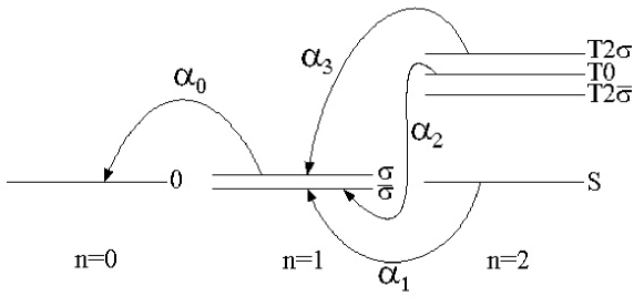
Figure 1: Quasiparticle excitations between state in full singlet-triplet model (excitations for only one spin projections are shown).

The t-t’-J model is derived by exclusion the intersubband hopping between low (LHB) and upper (UHB) Hubbard subbands for the Hubbard model [11] and for 3-band p-d model [12]. We write the Hamiltonian in the form

$$H=H_{0}+H_{1},$$ (8)

where the excitations via the charge transfer gap are included in $H_{1}$. Then we define an operator

$$H\left(\epsilon\right)=H_{0}+\epsilon H_{1}$$ (9)

and make the unitary transformation

$$\tilde{H}\left(\epsilon\right)=\exp{\left(-\rmi\epsilon\hat{S}\right)}H\left(\epsilon\right)\,\exp{\left(\rmi\epsilon\hat{S}\right)}.$$ (10)

Vanishing linear in $\epsilon$ component of $\tilde{H}\left(\epsilon\right)$ gives the equation for matrix $\hat{S}$:

$$H_{1}+\rmi\left[H_{0},\hat{S}\right]=0.$$ (11)

The effective Hamiltonian is obtained in second order in $\epsilon$ and at $\epsilon=1$ is given by:

$$\tilde{H}=H_{0}+\frac{1}{2}\rmi\left[H_{1},\hat{S}\right].$$ (12)

It is convenient to express the matrix $\hat{S}$ in terms of X-operators [13]. Thus, for the multiband p-d model (1) with electron doping (n-type systems) we obtain the usual t-J model:

$$H_{t-J}=\sum_{i,\sigma}\varepsilon_{1}X_{i}^{\sigma\sigma}+\sum_{<i,j>,\sigma}t_{ij}^{00}X_{i}^{\sigma 0}X_{j}^{0\sigma}+\frac{1}{2}\sum_{<i,j>}J_{ij}\left(\vec{S}_{i}\vec{S}_{j}-\frac{1}{4}n_{i}n_{j}\right),$$ (13)

where spin operators $\vec{S}_{f}$ and number of particles operators $n_{f}$ can be expressed in terms of Hubbard operators as follows:

$$\vec{S}_{i}\vec{S}_{j}-\frac{1}{4}n_{i}n_{j}=\frac{1}{2}\sum_{\sigma}\left(X_{i}^{\sigma\bar{\sigma}}X_{j}^{\bar{\sigma}\sigma}-X_{i}^{\sigma\sigma}X_{j}^{\bar{\sigma}\bar{\sigma}}\right).$$ (14)

For p-type systems effective Hamiltonian has the form of a singlet-triplet t-t’-J model [13]:

$$\tilde{H}=H_{0}+H_{t}+H_{J},$$ (15)

where $H_{0}$ (unperturbated part of the Hamiltonian), $H_{t}$ (kinetic part of $\tilde{H}$) and $H_{J}$ (exchange part of $\tilde{H}$) are given by the following expressions:

$$H_{0}=\sum_{i}\left(\varepsilon_{1}\sum_{\sigma}X_{i}^{\sigma\sigma}+\varepsilon_{2S}X_{i}^{SS}+\varepsilon_{2T}\sum_{M}X_{i}^{TMTM}\right),$$ (16)

$$H_{t}=\sum_{<i,j>,\sigma}t_{ij}^{bb}X_{i}^{S\bar{\sigma}}X_{j}^{\bar{\sigma}S}+\sum_{<i,j>,\sigma}t_{fg}^{aa}\left(\sigma\sqrt{2}X_{i}^{T0\ \bar{\sigma}}-X_{i}^{T2\sigma\ \sigma}\right)\left(\sigma\sqrt{2}X_{j}^{\bar{\sigma}\ T0}-X_{j}^{\sigma\ T2\sigma}\right)$$

$$\hbox to0.0pt{\hss${}+{}$}\sum_{<i,j>,\sigma}t_{ij}^{ab}2\sigma\gamma_{b}\left[X_{i}^{S\bar{\sigma}}\left(\sigma\sqrt{2}X_{j}^{\bar{\sigma}\ T0}-X_{j}^{\sigma\ T2\sigma}\right)+H.c.\right],$$ (17)

$$H_{J}=\frac{1}{2}\sum_{<i,j>}\left(J_{ij}+\delta J_{ij}\right)\left(\vec{S}_{i}\vec{S}_{j}-\frac{1}{4}n_{i}n_{j}\right)-\frac{1}{2}\sum_{<i,j>,\sigma}\delta J_{ij}X_{i}^{\sigma\sigma}X_{j}^{\sigma\sigma}.$$ (18)

The $J_{ij}$ is the exchange integral:

$$J_{ij}=4\frac{\left(t_{ij}^{0b}\right)^{2}}{E_{ct}},$$ (19)

and $\delta J_{ij}$ is the correction to it (dependent on the triplet’s contribution):

$$\delta J_{ij}=2\upsilon^{2}\frac{\left(t_{ij}^{ab}\right)^{2}}{E_{ct}}.$$ (20)

For the nearest neighbors ($i=0$, $j=1$) the estimation gives:

$$\frac{\delta J_{ij}}{J_{ij}}\sim 10^{-2}.$$ (21)

Here $E_{ct}$ is the charge-transfer energy gap (similar to $U$ in the Hubbard model, $E_{ct}\approx 2eV$ for cuprates).

Previously the motion of triplet holes and the simplest version of singlet-triplet model have been studied in [14, 15]. But these authors used the 3-band p-d model [1, 2] where the difference between energy of singlet and energy of triplet $\varepsilon_{T}-\varepsilon_{S}$ is about 2 eV. This fact leads to negligible contribution of singlet-triplet excitations in low-energy physics. But in multiband p-d model $\varepsilon_{T}-\varepsilon_{S}$ depends strongly on various model parameters, particularly on distance of apical oxygen ($p_{z}$-orbitals) from planar oxygen ($p_{x}$- and $p_{y}$-orbitals), energy of apical oxygen, difference between energy of $d_{z^{2}}$-orbitals and $d_{x^{2}-y^{2}}$-orbitals ($\varepsilon_{d_{z^{2}}}-\varepsilon_{d_{x^{2}-y^{2}}}$). For the realistic values of model parameters $\varepsilon_{T}-\varepsilon_{S}$ appears to be less or equal to 0.5 eV (see [3] and [10]). It is this small value of singlet-triplet splitting that let us believe that singlet-triplet excitations has a non-negligible contribution to band structure and also can give new superconducting pairing channel.

As easily can be noted the resulting Hamiltonian (15) is the generalization of t-J model to account of two-particle triplet state. But the inclusion of this triplet leads to such significant changes in Hamiltonian as renormalization of exchange integral (20) and appearing of $X_{i}^{\sigma\sigma}X_{j}^{\sigma\sigma}$ term in $H_{J}$.

More significant feature of effective singlet-triplet model (15) is the asymmetry for n- and p-type systems. This fact is known experimentally. In particular, the holes suppress antiferromagnetism more strongly than electrons. It was observed in $La_{2-x}Sr_{x}CuO_{4}$ in compare with $Nd_{2-x}Ce_{x}CuO_{4}$ [16]. For n-type systems the usual t-J model takes place while for p-type superconductors with complicated structure on the top of the valence band the singlet-triplet transitions plays an important role. In first case we have spin-fluctuation pairing mechanism (see review [17]). In the second case in addition to spin-fluctuations described by $H_{J}$ we also have pairing mechanism due to singlet-triplet excitations. Really, let’s look at structure of $H_{t}$. There we can see terms like $X_{i}^{S\,\bar{\sigma}}X_{j}^{\bar{\sigma}\,T0}$ which can be identically written according to multiplication rule of Hubbard operators:

$$X_{i}^{S\bar{\sigma}}X_{j}^{\bar{\sigma}T0}=X_{i}^{S\bar{\sigma}}X_{j}^{\bar{\sigma}S}X_{j}^{ST0}.$$ (22)

Here we can see three processes: creation ($X_{i}^{S\bar{\sigma}}$) and annihilation ($X_{j}^{\bar{\sigma}S}$) of the hole at different sites i and j, and spin-exciton $X_{j}^{ST0}$. This spin-exciton can play a role of intermediate boson in superconducting pairing.

3 Green Functions for Effective Singlet-Triplet Model

Processes described by Hamiltonian (15) are shown in the figure 2. We have three Fermi-type excitations and hence three base root vectors $\alpha_{1}$, $\alpha_{2}$, $\alpha_{3}$. Corresponding basis of the Hubbard operators is:

$$\left\{X_{i}^{\bar{\sigma}S},X_{i}^{\bar{\sigma}\ T0},X_{i}^{\sigma\ T2\sigma}\right\}\Rightarrow\left\{X_{i}^{1},X_{i}^{2},X_{i}^{3}\right\}.$$ (23)

The condition of basis completeness has a form:

$$\sum_{\sigma}X_{f}^{\sigma\sigma}+X_{f}^{SS}+\sum_{M}X_{f}^{TM\ TM}=1,$$ (24)

where $M=\left\{2\sigma,\ 0,\ 2\bar{\sigma}\right\}$.

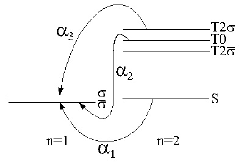
Figure 2: Quasiparticle excitations between state in effective singlet-triplet model (excitations for only one spin projections are shown).

In the introduced notations $H_{t}$ has the following form:

$$H_{t}=\sum_{<i,j>,\sigma}\sum_{m,n}\gamma_{ij,\sigma}(m,n)\,{X_{i\sigma}^{m}}^{+}X_{j\sigma}^{n},$$ (25)

where $m$ and $n$ are root vectors. Also, for further convenience, direct dependence on spin $\sigma$ is introduced. Matrix $\gamma_{ij,\,\sigma}(m,n)$ can easily be obtained from Hamiltonian (15):

$$\gamma_{ij,\sigma}(m,n)=\left(\begin{array}[]{ccc}t_{ij}^{bb}&\frac{1}{\sqrt{2}}\gamma_{b}t_{ij}^{ab}&-2\sigma\gamma_{b}t_{ij}^{ab}\\ \frac{1}{\sqrt{2}}\gamma_{b}t_{ij}^{ab}&\frac{1}{2}t_{ij}^{aa}&-\sigma\sqrt{2}t_{ij}^{aa}\\ -2\sigma\gamma_{b}t_{ij}^{ab}&-\sigma\sqrt{2}t_{ij}^{aa}&t_{ij}^{aa}\end{array}\right),$$ (26)

Equations of motion for Hamiltonian (15) can be expressed as:

$$\rmi\frac{\rmd}{\rmd t}X_{f\sigma}^{p}=\left[X_{f\sigma}^{p},H_{0}+H_{t}+H_{J}\right]=\Omega_{p}X_{f\sigma}^{p}+L_{f\sigma}^{p},$$ (27)

where $L_{f\sigma}^{p}=L_{f\sigma}^{p}(t)+L_{f\sigma}^{p}(J)$, $L_{f\sigma}^{p}(t)\equiv[X_{f\sigma}^{p},H_{t}]$, $L_{f\sigma}^{p}(J)\equiv[X_{f\sigma}^{p},H_{J}]$, and $\Omega_{p}\equiv[X_{f\sigma}^{p},H_{0}]$ is vector of one-electronic energies:

$$\Omega_{p}=\left(\begin{array}[]{l}\varepsilon_{2S}-\varepsilon_{1}\\ \varepsilon_{2T}-\varepsilon_{1}\\ \varepsilon_{2T}-\varepsilon_{1}\end{array}\right).$$ (28)

Taking into account equation (25) and identity $\left[A,BC\right]\equiv\left\{A,B\right\}C-B\left\{A,C\right\}$ we can right away get an expression for $L_{f\sigma}^{p}(t)$:

$$L_{f\sigma}^{p}(t)=\sum_{g,\sigma^{\prime}}\sum_{m,n}\gamma_{fg,\sigma^{\prime}}(m,n)\left(E_{f}^{\sigma\sigma^{\prime}}(p,m)X_{g\sigma^{\prime}}^{n}-{X_{g\sigma^{\prime}}^{m}}^{+}D_{f}^{\sigma\sigma^{\prime}}(p,n)\right),$$ (29)

where $E_{f}^{\sigma\sigma^{\prime}}(p,m)\equiv\left\{X_{f\sigma}^{p},{X_{f\sigma^{\prime}}^{m}}^{+}\right\}$ is the neutral boson and $D_{f}^{\sigma\sigma^{\prime}}(p,n)\equiv\left\{X_{f\sigma}^{p},X_{f\sigma^{\prime}}^{n}\right\}$ is $2e$ charged boson:

$$E_{f}^{\sigma\sigma^{\prime}}(p,m)=\delta_{\sigma\sigma^{\prime}}\left(\begin{array}[]{ccc}X_{f}^{SS}+X_{f}^{\bar{\sigma}\bar{\sigma}}&X_{f}^{ST0}&0\\ X_{f}^{T0S}&X_{f}^{T0T0}+X_{f}^{\bar{\sigma}\bar{\sigma}}&0\\ 0&0&X_{f}^{T2\sigma T2\sigma}+X_{f}^{\sigma\sigma}\end{array}\right)$$ (33)

$$\hbox to0.0pt{\hss${}+{}$}\delta_{\bar{\sigma}\sigma^{\prime}}\left(\begin{array}[]{ccc}X_{f}^{\bar{\sigma}\sigma}&0&X_{f}^{ST2\sigma}\\ 0&X_{f}^{\bar{\sigma}\sigma}&X_{f}^{T0T2\sigma}\\ X_{f}^{T2\bar{\sigma}S}&X_{f}^{T2\bar{\sigma}T0}&0\end{array}\right),$$ (37)

$$D_{f}^{\sigma\sigma^{\prime}}(p,n)=0.$$ (38)

Vanishing of $D_{f}^{\sigma\sigma^{\prime}}(p,n)$ is due to neglect of two-hole excitations $|0\rangle\rightarrow|S\rangle$ in the t-t’-J model. Nevertheless such excitations had their effect resulting in the superexchange interaction J.

It’s easy to rewrite expression for $L_{f\sigma}^{p}(t)$ in reciprocal space (or so-called k-space):

$$L_{k\sigma}^{p}(t)=\sum_{q,\sigma^{\prime}}\sum_{m,n}\gamma_{-q,\sigma^{\prime}}(m,n)E_{k-q}^{\sigma\sigma^{\prime}}(p,m)X_{q\sigma^{\prime}}^{n}.$$ (39)

Introducing for convenience operator:

$$Y_{q\sigma}\equiv\frac{1}{2}J_{-q}X_{q}^{\sigma\sigma}+\delta J_{-q}X_{q}^{\bar{\sigma}\bar{\sigma}},$$ (40)

we can now write down $L_{f\sigma}^{p}(J)$:

$$L_{k\sigma}^{1}(J)=\frac{1}{2}\sum_{q}\left(X_{k-q}^{\bar{\sigma}S}Y_{q\sigma}+Y_{q\sigma}X_{k-q}^{\bar{\sigma}S}-\frac{1}{2}J_{-q}\left(X_{k-q}^{\sigma S}X_{q}^{\bar{\sigma}\sigma}+X_{q}^{\bar{\sigma}\sigma}X_{k-q}^{\sigma S}\right)\right),$$ (41)

$$L_{k\sigma}^{2}(J)=\frac{1}{2}\sum_{q}\left(X_{k-q}^{\bar{\sigma}\ T0}Y_{q\sigma}+Y_{q\sigma}X_{k-q}^{\bar{\sigma}\ T0}-\frac{1}{2}J_{-q}\left(X_{k-q}^{\sigma\ T0}X_{q}^{\bar{\sigma}\sigma}+X_{q}^{\bar{\sigma}\sigma}X_{k-q}^{\sigma\ T0}\right)\right),$$ (42)

$$L_{k\sigma}^{3}(J)=\frac{1}{2}\sum_{q}\left(X_{k-q}^{\sigma\ T2\sigma}Y_{q\bar{\sigma}}+Y_{q\bar{\sigma}}X_{k-q}^{\sigma\ T2\sigma}-\frac{1}{2}J_{-q}\left(X_{k-q}^{\bar{\sigma}\ T2\sigma}X_{q}^{\sigma\bar{\sigma}}+X_{q}^{\sigma\bar{\sigma}}X_{k-q}^{\bar{\sigma}\ T2\sigma}\right)\right).$$ (43)

For decoupling of equations on Green functions we will use the method of irreducible operators [18]. This method based on linearization of equations of motion within Generalized Hartree-Fock Approximation (GHFA). Let us first introduce the irreducible operator:

$$\overline{L_{k\sigma}^{p}}=L_{k\sigma}^{p}-\sum_{h}C_{k\sigma}(p,h)X_{k\sigma}^{h}-\sum_{h}\Delta_{k\sigma}(p,h){X_{-k\bar{\sigma}}^{h}}^{+},$$ (44)

where

$$C_{k\sigma}(p,h)=\frac{\left\langle\left\{L_{k\sigma}^{p},{X_{k\sigma}^{h}}^{+}\right\}\right\rangle}{\left\langle\left\{X_{k\sigma}^{h},{X_{k\sigma}^{h}}^{+}\right\}\right\rangle},$$ (45)

$$\Delta_{k\sigma}(p,h)=\frac{\left\langle\left\{L_{k\sigma}^{p},X_{-k\bar{\sigma}}^{h}\right\}\right\rangle}{\left\langle\left\{{X_{-k\bar{\sigma}}^{h}}^{+},X_{-k,\bar{\sigma}}^{h}\right\}\right\rangle}.$$ (46)

Here $\Delta_{k\sigma}$ connected to the superconducting order parameter. Its symmetrical properties will be analyzed in next chapter.

Now we can write down expressions for $C_{k\sigma}(p,h)$ and $\Delta_{k\sigma}(p,h)$ in compact form:

$$C_{k\sigma}(p,h)=\frac{1}{\left\langle E_{k=0}^{\sigma\sigma}(h,h)\right\rangle}\sum_{q}\left\langle E_{q}^{\sigma\sigma}(h,h)\right\rangle$$

$$\hbox to0.0pt{\hss${}\times{}$}\left[\gamma_{q-k,\sigma}(p,h)\left\langle E_{-q}^{\sigma\sigma}(p,p)\right\rangle+\delta_{p,h}\left\langle Y_{-q\sigma}(p,h)\right\rangle\right],$$ (47)

$$\Delta_{k\sigma}(p,h)=\frac{1}{\left\langle E_{k=0}^{\bar{\sigma}\bar{\sigma}}(h,h)\right\rangle}\sum_{q}\left[-A_{q-k}^{(1)}(p,h)B_{q\sigma}(h,p)-A_{q+k}^{(2)}(p,h)B_{q\sigma}(p,h)\right.$$

$$\hbox to0.0pt{\hss${}+{}$}\left.\sum_{m,n}\left(\gamma_{-q,\sigma}(m,n)R_{q\sigma}^{(1)}(p,m;h,n)-\gamma_{-q,\bar{\sigma}}(m,n)R_{q\sigma}^{+(2)}(p,m;h,n)\right)\right].$$ (48)

Tensors $R_{q\sigma}^{(1)}(p,m;h,n)$ and $R_{q\sigma}^{+\,(2)}(p,m;h,n)$ are presented in A.

Averaging-out in $C_{k\sigma}(p,h)$ were made in Hubbard-I approximation and all averages in $C_{k\sigma}(p,h)$ are as follows:

$$\left\langle E_{k}^{\sigma\sigma^{\prime}}(p,h)\right\rangle=\delta_{\sigma\sigma^{\prime}}\left(\begin{array}[]{ccc}\left\langle X_{k}^{SS}+X_{k}^{\bar{\sigma}\bar{\sigma}}\right\rangle&0&0\\ 0&\left\langle X_{k}^{T0T0}+X_{k}^{\bar{\sigma}\bar{\sigma}}\right\rangle&0\\ 0&0&\left\langle X_{k}^{T2\sigma T2\sigma}+X_{k}^{\sigma\sigma}\right\rangle\end{array}\right),$$ (52)

$$\left\langle Y_{q\sigma}(p,h)\right\rangle=\left(\begin{array}[]{ccc}\left\langle Y_{q\sigma}\right\rangle&0&0\\ 0&\left\langle Y_{q\sigma}\right\rangle&0\\ 0&0&\left\langle Y_{q\bar{\sigma}}\right\rangle\end{array}\right),$$ (56)

where $Y_{q\sigma}$ is determined by (40). Also the anomalous averages were introduced:

$$B_{k\sigma}(p,h)\equiv\left\langle X_{-k\bar{\sigma}}^{p}X_{k\sigma}^{h}\right\rangle.$$ (57)

Direct calculations can reveal one useful property of this averages:

$$B_{-k\bar{\sigma}}(h,p)=-B_{k\sigma}(p,h).$$ (58)

At calculation of $\left\langle\left\{L_{k\sigma}^{3}(J),X_{-k\bar{\sigma}}^{h}\right\}\right\rangle$ the terms of type $\left\langle X_{k-q}^{\bar{\sigma}\ T2\sigma}P_{k,q}^{\sigma}(h)\right\rangle$ appears where $P_{k,q}^{\sigma}(h)=\sqrt{N}[X_{q}^{\bar{\sigma}\sigma},X_{-k\bar{\sigma}}^{h}]$ is a Fermi-like operator. These terms are responsible for 3-fermion excitations and in the Hubbard-I approximation they are equal to zero.

Tensors $R_{q\sigma}^{(1)}(p,m;h,n)$ and $R_{q\sigma}^{+\,(2)}(p,m;h,n)$ are presented in Appendix I. Shortly, each of their elements is equal to anomalous average $B_{q\sigma}$ or zero. Matrixes $A_{q-k}^{(1)}(p,h)$ and $A_{q+k}^{(2)}(p,h)$ consist of exchange integrals and has the following explicit form:

$$A_{q-k}^{(1)}(p,h)=\frac{1}{2}\left(\begin{array}[]{ccc}J_{q-k}&J_{q-k}&2\delta J_{q-k}\\ J_{q-k}&J_{q-k}&2\delta J_{q-k}\\ 2\delta J_{q-k}&2\delta J_{q-k}&2\delta J_{q-k}\end{array}\right),$$ (62)

$$A_{q+k}^{(2)}(p,h)=\frac{1}{2}\left(\begin{array}[]{ccc}J_{q+k}&J_{q+k}&0\\ J_{q+k}&J_{q+k}&0\\ 0&0&0\end{array}\right).$$ (66)

We can now perform elementary check of the obtained $\Delta_{k\sigma}(p,h)$ and $C_{k\sigma}(p,h)$ by using fact that when moving energy of the triplet $TM$ to the infinity we have to obtain the usual t-J model [19, 20]. Because in paper [19] Hubbard operators were also used we will compare our gap and renormalization of spectrum with its results:

$$C_{k\sigma}^{t-J}=t_{k}(1-n_{\bar{\sigma}})-\frac{J}{2}n_{\bar{\sigma}},$$ (67)

$$\Delta_{k\sigma}^{t-J}=\frac{1}{1-n_{\sigma}}\sum_{q}\left(2t_{q}-\frac{1}{2}\left(J_{k+q}+J_{k-q}\right)\right)B_{q\sigma}^{t-J}.$$ (68)

Neglecting all excitations to the triplet zone ($\alpha_{2}\rightarrow 0$, $\alpha_{3}\rightarrow 0$, $\delta J_{q}\rightarrow 0$, and $t_{fg}^{nm}\rightarrow 0$ if n or m is equal to a) coefficients and matrixes in singlet-triplet model becomes:

$$\gamma_{fg,\sigma}(m,n)=\delta_{m1}\delta_{n1}t_{fg}^{bb},$$ (69)

$$\left\langle E_{f}^{\sigma\sigma^{\prime}}\right\rangle=\delta_{p1}\delta_{m1}\delta_{\sigma,\sigma^{\prime}}\left\langle X_{f}^{SS}+X_{f}^{\bar{\sigma}\bar{\sigma}}\right\rangle,$$ (70)

$$B_{q\sigma}(p,h)=\delta_{p1}\delta_{h1}\left\langle X_{-q\bar{\sigma}}^{1}X_{q\sigma}^{1}\right\rangle\equiv B_{q\sigma},$$ (71)

$$\left\langle Y_{q\sigma}(p,h)\right\rangle=\delta_{p1}\delta_{h1}\left\langle\frac{1}{2}J_{-q}X_{q}^{\sigma\sigma}\right\rangle.$$ (72)

Having made all these limiting transitions in (47) and (48) we derive:

$$C_{k\sigma}\rightarrow\frac{1}{1-n_{\bar{\sigma}}}\sum_{q}(1-n_{\bar{\sigma}})\left(t_{q-k}^{bb}(1-n_{\bar{\sigma}})+\frac{1}{2}J_{-q}(-n_{\bar{\sigma}})\right)\delta_{q,0}$$

$$\hbox to0.0pt{\hss${}={}$}t_{k}^{bb}(1-n_{\bar{\sigma}})-\frac{1}{2}J_{0}n_{\bar{\sigma}},$$ (73)

$$\Delta_{k\sigma}\rightarrow\frac{1}{1-n_{\sigma}}\sum_{q}\left(2t_{-q}^{bb}-\frac{1}{2}\left(J_{q-k}+J_{q+k}\right)\right)B_{q\sigma}.$$ (74)

This is exactly what we have in the t-J model. So the effective singlet-triplet model in the low energy limit (triplet energy tend to infinity) reduces to the t-J model.

Let’s return to decoupling of Green functions. In GHFA we have to put irreducible operator $\overline{L_{k\sigma}^{p}}$ to zero. In this case the equations of motion take the following form:

$$\cases{\rmi\frac{\rmd}{\rmd t}X_{k\sigma}^{p}=\sum_{h}\left[\Omega_{p}\ \delta_{p,h}+C_{k\sigma}(p,h)\right]X_{k\sigma}^{h}+\sum_{h}\Delta_{k\sigma}(p,h){X_{-k\bar{\sigma}}^{h}}^{+}\\ \rmi\frac{\rmd}{\rmd t}{X_{-k\bar{\sigma}}^{p}}^{+}=-\sum_{h}\left[\Omega_{p}\ \delta_{p,h}+C_{-k\bar{\sigma}}^{+}(p,h)\right]{X_{-k\bar{\sigma}}^{h}}^{+}-\sum_{h}\Delta_{-k\bar{\sigma}}^{+}(p,h)X_{k\sigma}^{h}}$$ (75)

Now we can easily write down a system of Gorkov type equations for normal and abnormal, and this system is closed:

$$\cases{\sum_{h}\left[\left(E-\Omega_{p}\right)\delta_{p,h}-C_{k\sigma}(p,h)\right]\hat{G}_{k\sigma}(h,l)-\sum_{h}\Delta_{k\sigma}(p,h)\hat{F}_{k\sigma}^{+}(h,l)=\left\langle\left\{X_{k\sigma}^{p},{X_{k\sigma}^{l}}^{+}\right\}\right\rangle\\ \sum_{h}\left[\left(E+\Omega_{p}\right)\delta_{p,h}+C_{-k\bar{\sigma}}^{+}(p,h)\right]\hat{F}_{k\sigma}^{+}(h,l)+\sum_{h}\Delta_{-k\bar{\sigma}}^{+}(p,h)\hat{G}_{k\sigma}(h,l)=0}$$ (76)

Actually this is an equation for a matrix normal Green function $\hat{G}_{k\sigma}=\left\langle\left\langle X_{k\sigma}^{h}\right.\left|{X_{k\sigma}^{l}}^{+}\right\rangle\right\rangle$ and matrix abnormal Green function $\hat{F}_{k\sigma}^{+}=\left\langle\left\langle{X_{-k\bar{\sigma}}^{h}}^{+}\right.\left|{X_{k\sigma}^{l}}^{+}\right\rangle\right\rangle$.

Introducing matrixes:

$$\hat{\Re}_{k\sigma}=\left(\Omega_{p}\delta_{p,h}+C_{k\sigma}(p,h)\right),$$ (77)

$$\hat{\Delta}_{k\sigma}=\Delta_{k\sigma}(p,h),$$ (78)

$$\hat{E}_{k}^{\sigma\sigma}=E_{k}^{\sigma\sigma}(p,h)\equiv\sqrt{N}\left\{X_{k\sigma}^{p},{X_{k\sigma}^{l}}^{+}\right\},$$ (79)

and solving equations we obtain expressions for $\hat{G}_{k\sigma}$ and $\hat{F}_{k\sigma}^{+}$:

$$\cases{\hat{F}_{k\sigma}^{+}=-\left[E\hat{I}+\hat{\Re}_{-k\bar{\sigma}}^{+}\right]^{-1}\hat{\Delta}_{-k\bar{\sigma}}^{+}\hat{G}_{k\sigma}\\ \hat{G}_{k\sigma}=\left[E\hat{I}-\hat{\Re}_{k\sigma}+\hat{\Delta}_{k\sigma}\left(E\hat{I}+\hat{\Re}_{-k\bar{\sigma}}^{+}\right)^{-1}\hat{\Delta}_{-k\bar{\sigma}}^{+}\right]^{-1}\left\langle\hat{E}_{k}^{\sigma\sigma}\right\rangle/\sqrt{N}}$$ (80)

where $\hat{I}$ is identity matrix and N is number of vectors in k-space.

It can be seen now by analogy with the BCS theory of low-temperature superconductivity that $\Delta_{k\sigma}$ is the superconducting order parameter.

The system (80) is the set of matrix Green function and can be used to obtain energy spectrum and averages for any problem with defined basis of root vectors. In following chapters we will use system (80) to perform symmetry classification of order parameter and to investigate normal paramagnetic phase.

4 Symmetry Classification of Superconducting Order Parameter

An early suggestion that AF spin fluctuation could give rise to singlet $d_{x^{2}-y^{2}}$- wave pairing in p-type cuprate superconductors was made by Bickers, Scalapino and Scalettar [21]. This suggestion has been supported by the FLEX approximation to the Hubbard model [22] that is, however not valid in the case of $U\gg t$. In this limit of SCES the proper model is the t-J model. Exact diagonalization and quantum Monte-Carlo method results for small clusters have been discussed by Dagotto [23]. For the infinite lattice the most adequate perturbation approach to the t-J model has been formulated in the X-operator representation because of the exact treatment of local constraint due to X-operators algebra. The mean-field solution [24, 25, 26] of the t-J model and analysis of the self-energy correlations beyond the mean-field approximation by diagram technique [27] and by high-order decoupling scheme [20] has confirmed the $d_{x^{2}-y^{2}}$- pairing in the hole-doped system with typical $T_{c}(x)$ dependence. Latest experimental results appear to prove $d_{x^{2}-y^{2}}$- pairing not only in p-type systems but also in n-type systems (see review [28]).

Let’s proceed to a symmetry classification of the order parameter $\Delta_{k\sigma}(p,h)$ in the effective singlet-triplet model considering case of square lattice. First, we have to break hopping and exchange integrals in two terms:

$$\gamma_{k}(p,h)=t(p,h)\omega_{k}+t^{\prime}(p,h)\tilde{\omega}_{k},$$ (81)

$$J_{k}=J\omega_{k}+J^{\prime}\tilde{\omega}_{k},$$ (82)

$$\delta J_{k}=\delta J\omega_{k}+\delta J^{\prime}\tilde{\omega}_{k},$$ (83)

where

$$\omega_{k} = \sum_{\delta}\exp{\left(\rmi k\delta\right)}=2\left(\cos k_{x}+\cos k_{y}\right),$$ (84)

$$\tilde{\omega}_{k} = \sum_{\delta^{\prime}}\exp{\left(\rmi k\delta^{\prime}\right)}=4\cos k_{x}\cos k_{y},$$ (85)

and non-primed values are concerned with nearest neighbor (figure 3(a), first coordination sphere) and primed values are concerned with next-nearest neighbor (figure 3(b), second coordination sphere).

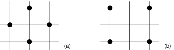
Figure 3: Location of nearest neighbors (a) and next-nearest neighbors (b) on square lattice.

Second, to make a classification we will distinguish following symmetry types:

4.1 s-type

In superconducting phase we have a constraint condition:

$$\frac{1}{N}\sum_{k}\left\langle a_{k\sigma}a_{-k\bar{\sigma}}\right\rangle=0.$$ (86)

Right side of this identity in the effective singlet-triplet model is equal to zero due to choose of basis of root vectors $\alpha_{i}$, i.e. because of absence of the transitions from lower to higher Hubbard bands. Moreover, condition (86) is satisfied only in case of p- and d-pairing but not for symmetric s-pairing. Hence in the singlet-triplet model the symmetric s-type singlet pairing is absent.

4.2 p-type

Triplet pairing of p-type is impossible because for realization of this symmetry there must be a ferromagnetic interaction (see e.g. [19]) but in case of singlet-triplet model we have only antiferromagnetic exchange.

4.3 d-type

Singlet d-type pairing is forbidden neither by the constraint condition (86) nor by the type of interaction.

First consider $d_{x^{2}-y^{2}}$- pairing type. In this case there is a restriction:

$$\sum_{q}\cos q_{x}B_{q\sigma}(p,h)=-\sum_{q}\cos q_{y}B_{q\sigma}(p,h),$$ (87)

and, as a consequence,

$$\sum_{q}\sin q_{x}B_{q}=0,$$ (88)

and

$$\sum_{q}\sin q_{y}B_{q}=0.$$ (89)

This immediately leads to the significant simplification of superconducting gap $\Delta_{k\sigma}(p,h)\equiv\Delta_{k\sigma}^{(d_{x^{2}-y^{2}})}(p,h)$:

$$\Delta_{k\sigma}^{(d_{x^{2}-y^{2}})}(p,h)=-\frac{2\Delta_{\sigma}^{(d_{x^{2}-y^{2}})}(p,h)}{\sqrt{N}\left\langle E_{k=0}^{\bar{\sigma}\bar{\sigma}}(h,h)\right\rangle}(\cos k_{x}-\cos k_{y}).$$ (90)

where $\Delta_{\sigma}^{(d_{x^{2}-y^{2}})}(p,h)$ is the impulse-independent part of the gap:

$$\Delta_{\sigma}^{(d_{x^{2}-y^{2}})}\equiv\left(\begin{array}[]{ccc}J\Psi_{\sigma}^{1,1}&J\left(\Psi_{\sigma}^{1,2}+\Psi_{\sigma}^{2,1}\right)/2&\delta J\Psi_{\sigma}^{3,1}\\ J\left(\Psi_{\sigma}^{1,2}+\Psi_{\sigma}^{2,1}\right)/2&J\Psi_{\sigma}^{2,2}&\delta J\Psi_{\sigma}^{3,2}\\ \delta J\Psi_{\sigma}^{1,3}&\delta J\Psi_{\sigma}^{2,3}&\delta J\Psi_{\sigma}^{3,3}\end{array}\right),$$ (91)

$$\Psi_{\sigma}^{p,h}\equiv\sum_{q}(\cos q_{x}-\cos q_{y})B_{q\sigma}(p,h).$$ (92)

Impulse-independent $\Delta_{\sigma}^{(d_{x^{2}-y^{2}})}(p,h)$ includes exchange integrals only for nearest neighbors and therefore can exist only in boundaries of first coordination sphere.

Now lets consider $d_{xy}$- pairing type. The restriction made by this symmetry is as follows:

$$\sum_{q}\cos q_{x}\cos q_{y}B_{q\sigma}(p,h)=0.$$ (93)

Also

$$\sum_{q}\sin q_{x}\cos q_{y}B_{q}=0,$$ (94)

and

$$\sum_{q}\cos q_{x}\sin q_{y}B_{q}=0.$$ (95)

The superconducting gap $\Delta_{k\sigma}(p,h)\equiv\Delta_{k\sigma}^{(d_{xy})}(p,h)$ takes the form:

$$\Delta_{k\sigma}^{(d_{xy})}(p,h)=-\frac{4\Delta_{\sigma}^{(d_{xy})}(p,h)}{\sqrt{N}\left\langle E_{k=0}^{\bar{\sigma}\bar{\sigma}}(h,h)\right\rangle}\sin k_{x}\sin k_{y}.$$ (96)

where impulse-independent part of the gap $\Delta_{\sigma}^{(d_{xy})}(p,h)$:

$$\Delta_{\sigma}^{(d_{xy})}\equiv\left(\begin{array}[]{ccc}J^{\prime}\Phi_{\sigma}^{1,1}&J^{\prime}\left(\Phi_{\sigma}^{1,2}+\Phi_{\sigma}^{2,1}\right)/2&\delta J^{\prime}\Phi_{\sigma}^{3,1}\\ J^{\prime}\left(\Phi_{\sigma}^{1,2}+\Phi_{\sigma}^{2,1}\right)/2&J^{\prime}\Phi_{\sigma}^{2,2}&\delta J^{\prime}\Phi_{\sigma}^{3,2}\\ \delta J^{\prime}\Phi_{\sigma}^{1,3}&\delta J^{\prime}\Phi_{\sigma}^{2,3}&\delta J^{\prime}\Phi_{\sigma}^{3,3}\end{array}\right),$$ (97)

$$\Phi_{\sigma}^{p,h}\equiv\sum_{q}\sin q_{x}\sin q_{y}B_{q\sigma}(p,h).$$ (98)

Coexistence of $d_{x^{2}-y^{2}}$- and $d_{xy}$- pairing types is forbidden by the group theory: in the considered case of tetragonal lattice symmetry $d_{x^{2}-y^{2}}$- and $d_{xy}$- types belongs to different irreducible representation (see review [28]) so there must be concurrence between these types of pairing.

Note that triplet channel results in $\delta J$ in matrix (91) and $\delta J^{\prime}$ in matrix (97). Obviously triplet channel gives the additional pairing.

It is very interesting that $d_{xy}$-type includes exchange integrals only for next-nearest neighbors (see equation (97)) and therefore can exist only in second coordination sphere. Hence in nearest neighbor approximation we can have only order parameter of $d_{x^{2}-y^{2}}$-symmetry.

Actually equations (90) and (96) are equations for order parameters $\Psi_{\sigma}^{p,h}$ and $\Phi_{\sigma}^{p,h}$ respectively and should be solved self-consistently via Green function equations (80). When this is done we can obtain energy spectrum and phase diagram $T_{c}$ versus concentration $x$.

4.4 Other symmetry types

The other symmetry types are not realized due to absence of corresponding combinations of trigonometrical functions in expression for superconducting gap (48).

Combination of previously analyzed types such as s+d is impossible because in the considered case of tetragonal lattice symmetry s- and d- types belongs to different irreducible representation (see review [28] and references from there). So the order parameter symmetry must be of d-type or, more precisely, to be a concurrence of $d_{x^{2}-y^{2}}$ and $d_{xy}$ singlet pairing types. This conclusion is true not only for hole doped systems but also for electron doped systems because in the limit of infinite energy of singlet-triplet excitation (i.e. absence of excitations to the triplet states - this case corresponds to n-type cuprates) our equations take the form of t-J model ones and the gap symmetry remains.

5 Normal Paramagnetic Phase

In normal paramagnetic phase $\Delta_{k\sigma}=0$ and Green function equations (80) become essentially simpler:

$$\cases{\hat{G}_{k\sigma}=\left(E\hat{I}-\hat{\Re}_{k\sigma}\right)^{-1}\left\langle\hat{E}_{k}^{\sigma\sigma}\right\rangle/\sqrt{N}\\ \hat{F}_{k\sigma}^{+}=0}$$ (99)

By solving these equations one can obtain energy spectrum and self-consistently find Fermi level. Also using following definition for the spectral density in terms of one-electron annihilation operators $c_{k}^{+}$:

$$A(k,\sigma,E)=-\frac{1}{\pi}\mathrm{Im}\left\langle\left\langle c_{k\sigma}^{+}\right.\left|c_{k\sigma}\right\rangle\right\rangle,$$ (100)

we can calculate density of states (DOS):

$$N(E)=\frac{1}{N}\sum_{k\sigma}A(k,\sigma,E)=\frac{1}{N}\sum_{k,\sigma,\lambda}\left(-\frac{1}{\pi}\mathrm{Im}\left\langle\left\langle c_{k\sigma\lambda}^{+}\right.\left|c_{k\sigma\lambda}\right\rangle\right\rangle\right),$$ (101)

where $\sigma$ is spin and $\lambda$ is the orbital index. In terms of Hubbard operators the expression for DOS has the following explicit form:

$$N(E)=-\frac{1}{N}\sum_{k\sigma}\left[\left(\gamma_{x}^{2}+\gamma_{b}^{2}\right)\mathrm{Im}\left\langle\left\langle{X_{k\sigma}^{1}}^{+}\right.\left|X_{k\sigma}^{1}\right\rangle\right\rangle+\right.$$

$$\hbox to0.0pt{\hss${}+{}$}\left.\left(\gamma_{z}^{2}+\gamma_{a}^{2}+\gamma_{p}^{2}\right)\left(\frac{1}{2}\mathrm{Im}\left\langle\left\langle{X_{k\sigma}^{2}}^{+}\right.\left|X_{k\sigma}^{2}\right\rangle\right\rangle+\mathrm{Im}\left\langle\left\langle{X_{k\sigma}^{3}}^{+}\right.\left|X_{k\sigma}^{3}\right\rangle\right\rangle\right)\right]$$

$$\hbox to0.0pt{\hss${}={}$}\frac{1}{N}\sum_{k\sigma}\left[\left(\gamma_{x}^{2}+\gamma_{b}^{2}\right)\mathrm{Im}\hat{G}_{k\sigma}^{\mathrm{a}}(1,1)+\right.$$

$$\hbox to0.0pt{\hss${}+{}$}\left.\left(\gamma_{z}^{2}+\gamma_{a}^{2}+\gamma_{p}^{2}\right)\left(\frac{1}{2}\mathrm{Im}\hat{G}_{k\sigma}^{\mathrm{a}}(2,2)+\mathrm{Im}\hat{G}_{k\sigma}^{\mathrm{a}}(3,3)\right)\right].$$ (102)

Here $\epsilon$ and $N_{0}(\epsilon)$ is the dispersion and DOS for non-interacting case, $\gamma_{m}$ is the coefficient of transformation $c_{k\sigma}=\sum\limits_{m}\gamma_{m}X_{k\sigma}^{m}$, index ”$\mathrm{a}$” of Green function denotes that $\hat{G}_{k\sigma}^{\mathrm{a}}$ is advance Green function (while all over the paper we have used retarded Green functions). There is simple relation between this two types: $\hat{G}_{k\sigma}(p,h)=-\hat{G}_{k\sigma}^{\mathrm{a}}(h,p)$.

The calculations described above where performed for High-$T_{c}$ superconductor $La_{2-x}Sr_{x}CuO_{4}$ with the following set of the model parameters (in eV):

$t_{pd}=1$,	$\varepsilon(d_{x^{2}-y^{2}})=0$,	$\varepsilon(d_{z^{2}})=2$,	$\varepsilon(p_{x})=1.5$,	$\varepsilon(p_{z})=0.45$,
$t_{pp}=0.46$,	$t^{\prime}_{pp}=0.42$,	$U_{d}=9$, $U_{p}=4$,	$V_{pd}=1.5$,	$J_{d}=1$.

The same parameters where previously used in [10] for undoped $La_{2-x}Sr_{x}CuO_{4}$. The energy dispersion, obtained there, proved to be in good agreement with experimental ARPES data.

Our results for slightly overdoped copper oxide (concentration of dopant $x=0.2$) are presented in figure 4.

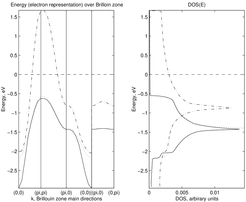
Figure 4: Energy Dispersion (on the left) and Density of States (on the right) in normal paramagnetic phase of the effective singlet-triplet model for concentration of dopant $x=0.2$. Energy of the singlet sub-band and its DOS are marked by dash-dotted line. Energy of the triplet sub-bands and corresponding DOS are marked by straight and dotted lines. Dashed line indicates location of the Fermi level.

Interesting case of coincidence of Fermi level and Van-Hove singularity is shown in figure 5.

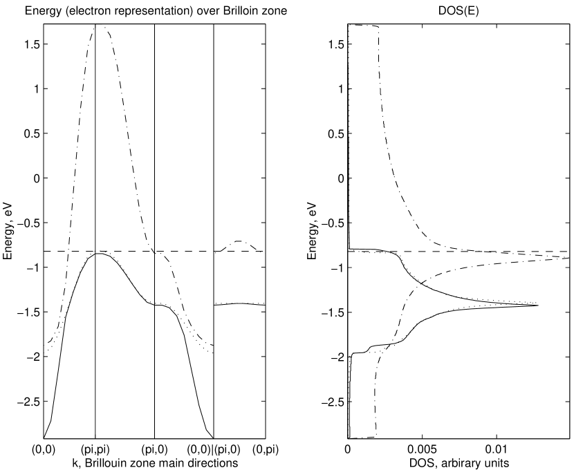
Figure 5: Energy Dispersion (on the left) and Density of States (on the right) in normal paramagnetic phase of the effective singlet-triplet model for concentration of dopant $x=0.43$. All definitions are the same as in figure 4. Distance between Van-Hove singularity and Fermi level is 0.074 eV

It can be seen that singlet sub-band is very wide - almost 3 eV. It is a consequence of Hubbard I approximation in spectrum renormalization term $C_{k\sigma}(p,h)$ (equation (47)). In more rigorous approximations with inclusion of spin correlators the energy bands should be more narrow (see [29] and [30]).

At the concentration $x=0.43$ Fermi level coincides with Van-Hove singularity in singlet sub-band. But if we will neglect hopping on second coordination sphere (nearest neighbor approximation) then we will get the flattening of dispersion in $(\pi,0)-(0,\pi)$ direction and shift of Van-Hove singularities to higher energies. This will result in coincidence of Fermi level and singularity in singlet sub-band at concentration $x=0.33$. It is typical value for the t-J model with nearest neighbor hopping t. It is also known that in t-t’-J model with the next-nearest neighbor hopping t’ the same shift in energies takes place so this phenomena is common both to t-t’-J model and the effective singlet-triplet model. Accepting the Van-Hove scenario of superconductivity, where the optimal doping correspond to coincident of Fermi level with Van-Hove singularity, we can clearly see that this should happened at $x=0.43$. Meanwhile the experimentally obtained optimal doping value for $La_{2-x}Sr_{x}CuO_{4}$ is $0.18$. So, either the Van-Hove scenario is not applicable or the model should be refined. This question could be answered only after the complete theory of superconductivity in the frame of the effective singlet-triplet model will be constructed.

6 Conclusion

In present work we obtained the effective Hamiltonian of the singlet-triplet model for copper oxides. Being the generalization of the t-J model to account of two-particle triplet state resulting Hamiltonian has several important features. At first, the $X_{i}^{\sigma\sigma}X_{j}^{\sigma\sigma}$ term appear which can have a non-trivial contribution to superconducting pairing. Second, the account of a triplet leads to renormalization of exchange integral. And third, the singlet-triplet model is asymmetric for n- and p-type systems. For n-type systems the usual t-J model takes place while for p-type superconductors with complicated structure on the top of the valence band the singlet-triplet transitions plays an important role. The asymmetry of p- and n-type systems is known experimentally.

The analysis of the possible processes in the effective singlet-triplet model shows that besides spin-fluctuation superconducting pairing mechanism typical for the t-J model we have pairing due to singlet-triplet transitions. These transitions induce spin-exciton which can play a role of intermediate boson in superconducting pairing.

We have also performed a symmetry classification of superconducting order parameter. It was shown that in case of tetragonal lattice s-type singlet pairing doesn’t take place while the $d_{x^{2}-y^{2}}$- and $d_{xy}$-types of singlet pairing can exist. Moreover, there must be a concurrence between $d_{x^{2}-y^{2}}$- and $d_{xy}$-types. At the same time, $d_{xy}$-type can exist only within the second coordination sphere and $d_{x^{2}-y^{2}}$-type can exist only within the first. This fact lets us to take into account only $d_{x^{2}-y^{2}}$-type symmetry of order parameter in nearest-neighbors approximation.

As concerns n-type cuprates, the gap symmetry was unclear for a long time. Recently, phase sensitive tunnel experiments by Tsuei and Kirtley [28] find an evidence for dominant $d_{x^{2}-y^{2}}$ symmetry in electron doped cuprates. This fact coincides with our results because in the limit of infinite energy of singlet-triplet excitation (i.e. absence of excitations to the triplet states - this case corresponds to n-type cuprates) our equations take the form of t-J model ones and the $d_{x^{2}-y^{2}}$-gap symmetry remain.

For normal paramagnetic phase we have obtained the energy dispersion over Brillouin zone and calculated density of states. Evolution of Fermi level with doping is also found. Both singlet and triplet excitations contributes to the density of states which leads to appearing of two Van-Hove singularities. At holes concentration $x=0.43$ the Fermi level crosses the first Van-Hove singularity corresponding to singlet sub-band. And at holes concentration $x=0.64$ the Fermi level crosses the second singularity corresponding to triplet sub-band.

7 Acknowledgements

The authors would like to thank N.M. Plakida and A.V. Sherman for discussions and useful comments.

This work has been supported by the RFBR grant 00-02-16110, by Krasnoyarsk Regional Science Foundation, grant 10F003C, by RFBR-”Enisey” grant 02-02-97705. INTAS support of research programme ”Electronic and magnetic properties in novel superconductors: spin fluctuations vs electron-phonon coupling” at number 654 is also acknowledged.

Appendix A Tensors $R_{q\sigma}^{(1)}(p,m;h,n)$ and $R_{q\sigma}^{+\,(2)}(p,m;h,n)$

Tensors $R_{q\sigma}^{(1)}(p,m;h,n)$ and $R_{q\sigma}^{+\,(2)}(p,m;h,n)$ where introduced as follows:

$$\sqrt{N}\left\langle[X_{-k\bar{\sigma}}^{h},E_{k-q}^{\sigma\sigma^{\prime}}(p,m)]X_{q\sigma^{\prime}}^{n}\right\rangle\equiv\delta_{\sigma\sigma^{\prime}}R_{q\sigma}^{(1)}(p,m;h,n)+\delta_{\bar{\sigma}\sigma^{\prime}}R_{q\bar{\sigma}}^{(2)}(p,m;h,n).$$ (103)

The ”+” symbol in $R_{q\sigma}^{+(2)}(p,m;h,n)$ means that all averages $B_{q\sigma}(p,h)$ in it has a interchanged indices p and h.

Table 1: $R_{q\sigma}^{(1)}(p,m;h,n)$

• 		m=1	m=2	m=3
  	h=1	$B_{q\sigma}(1,n)$	0	0
  p=1	h=2	0	$B_{q\sigma}(2,n)$	0
  	h=3	$-B_{q\sigma}(3,n)$	0	0
  	h=1	$B_{q\sigma}(2,n)$	0	0
  p=2	h=2	0	$B_{q\sigma}(2,n)$	0
  	h=3	0	$-B_{q\sigma}(3,n)$	0
  	h=1	0	0	$-B_{q\sigma}(1,n)$
  p=3	h=2	0	0	$-B_{q\sigma}(2,n)$
  	h=3	0	0	0

Table 2: $R_{q\sigma}^{+\,(2)}(p,m;h,n)$

• 		m=1	m=2	m=3
  	h=1	$-B_{q\sigma}(n,1)$	0	0
  p=1	h=2	$B_{q\sigma}(n,2)$	0	0
  	h=3	0	0	$B_{q\sigma}(n,1)$
  	h=1	0	$-B_{q\sigma}(n,1)$	0
  p=2	h=2	0	$-B_{q\sigma}(n,2)$	0
  	h=3	0	0	$B_{q\sigma}(n,2)$
  	h=1	$B_{q\sigma}(n,3)$	0	0
  p=3	h=2	0	$B_{q\sigma}(n,3)$	0
  	h=3	0	0	0

References

References

• [1] Emery V J 1987 Phys. Rev. Lett.58, 2794
• [2] Varma C M, Schmitt-Rink S, Abrahams E 1987 Solid State Commun.62, 681
• [3] Ovchinnikov S G 1996 JETP Letters 64, 25
• [4] Bianconi A, De Santis M, Di Cicco A et al1988 Phys. Rev.B 38, 7196
• [5] Gaididei Yu B, Loktev V M 1988 Phys. Status SolidiB 147, 307
• [6] Gavrichkov V A, Ovchinnikov S G 1998 Fizika Tverdogo Tela, 40, 184
• [7] Kamimura H, Eto M 1990 J. Phys. Soc. Japan59, 3053 (1990)
• [8] Eskes H, Tjeng L H, Sawatzky G A 1990 Phys. Rev.B 41, 1, 288
• [9] Ovchinnikov S G, Sandalov I S 1989 Physica C 161, 607
• [10] Gavrichkov V A, Ovchinnikov S G, Borisov A A, Goryachev E G 2000 JETP 91, 369
• [11] Chao K A, Spalek J, Oles A M 1977 J. Phys. C: Solid State Phys.10, 271
• [12] Belinicher V I, Chernyshev A I, Shubin V A 1996 Phys. Rev.B 53, 335
• [13] Korshunov M M, Ovchinnikov S G 2001 Phys. Solid State 43, 416
• [14] Zaanen J, Oles A M, Horsch P 1992 Phys. Rev.B 46, 5798
• [15] Hayn R, Yushannkhai V, Lotsov S 1993 Phys. Rev.B 47, 5253
• [16] Keimer B, Belk N, Birgeneau R J et al1992 Phys. Rev.B 46, 14034
• [17] Izyumov Yu A 1999 Physics Uspekhi 42, 215
• [18] Tyablikov S V 1975 Metody Kavntovoi Teorii Magnetizma (Moscow: ”Nauka”), p 528
• [19] Kuz’min E V, Ovchinnikov S G, Baklanov I O 2000 Phys. Rev.B 61, 15392
• [20] Plakida N M, Oudovenko V S 1999 Phys. Rev.B 59, 11949
• [21] Bickers N E, Scalapino D J, Scalettar R T 1987 Int. J. Mod. Phys. B 1, 687
• [22] Bickers N E, Scalapino D J, White S R 1989 Phys. Rev. Lett.62, 961
• [23] Dagotto E 1994 Rev. Mod. Phys.66, 763
• [24] Plakida N M, Yushannkhai V Yu, Stasyuk I V 1989 Physica C 160, 80
• [25] Yushannkhai V Yu, Plakida N M, Kalinay P 1991 Physica C 174, 401
• [26] Beenen J, Edwards D M 1995 Phys. Rev.B 52, 13636
• [27] Izyumov Yu A, Letfulov B M 1991 J. Phys.: Condens. Matter3, 5373
• [28] Tsuei C C, Kirtley J R 2000 Rev. Mod. Phys.72, 969
• [29] Plakida N M, Oudovenko V S 1997 Phys. Rev.B 55, R11997
• [30] Plakida N M, Oudovenko V S 1999 Phys. Rev.B 59, 11949