IMSC/2001/12/55 cond-mat/0112439
On the Emergence of the Microcanonical Description from a Pure State

Abstract

We study, in general terms, the process by which a pure state can “self-thermalize” and appear to be described by a microcanonical density matrix. This requires a quantum mechanical version of the Gibbsian coarse graining that conceptually underlies classical statistical mechanics. We introduce some extra degrees of freedom that are necessary for this. Interaction between these degrees and the system can be understood as a process of resonant absorption and emission of “soft quanta”. This intuitive picture allows one to state a criterion for when self thermalization occurs. This paradigm also provides a method for calculating the thermalization rate using the usual formalism of atomic physics for calculating decay rates. We contrast our prescription for coarse graining, which is somewhat dynamical, with the earlier approaches that are intrinsically kinematical. An important motivation for this study is the black hole information paradox.

1 Introduction

1.1 Motivation

Understanding the principles of Statistical Mechanics from first principles still remains a challenge [[4]-[36]] despite the monumental work by the pioneers like Boltzman, Poincare etc. According to the fundamental principles of statistical mechanics a macro-system starting from an arbitrary initial state eventually tends to a state of so called thermodynamic equilibrium. Inherent in this assertion is a certain irreversibility and one of the main issues has been the reconciliation of this with the fact that basic dynamics is reversible. In the case of Quantum Statistical Mechanics there are additional complications as the thermodynamic equilibrium state, which is described by a mixed density matrix can never be obtained from a pure density matrix under quantum mechanical evolution which is described by unitary transformations. This last issue is also the crux of the so called Quantum Measurement Problem. Interest in these issues has recently been rekindled from a most unexpected direction i.e the problems of black hole entropy and of the so called black hole information. In this section we briefly describe each of these to bring into focus the issues we address in the rest of the paper

1.2 Foundations of Quantum Statistical Mechanics

The questions discussed above lead naturally to questions about the basic postulate of quantum statistical mechanics(QSM). The postulate is that of equal a priori probabilities for all microstates in a given macrostate of definite energy. Equivalently, the density matrix of an ensemble whose energy lies in the range $E_{0}$ to $E_{0}+\Delta E$ is given by the identity matrix in the energy basis, suitably normalized as shown ($N$ is the number of states in the given energy interval):

$$\rho={1\over N}I\;\;\;E_{0}\leq E\leq E_{0}+\Delta E$$ (1.2.1)

and for $E$ not in this interval,

$$\rho=0$$

It is worth pointing out here that the standard derivation of the microcanonical distribution can not be carried over automatically to QSM. In classical statistical mechanics one derives the microcanonical distribution, by maximizing the entropy:

$$S=-k_{B}\int dX^{N}\rho(X^{N})log\rho(X^{N})$$ (1.2.2)

subject to

$$1=\int dX^{N}\rho(X^{N})$$ (1.2.3)

In these eqns $\rho(X^{N})$ is the distribution function on the phase space. The result one obtains is

$$\rho(X^{N})=const~{}~{}~{}~{}~{}E_{0}\leq H\leq E_{0}+\Delta E$$ (1.2.4)

and zero otherwise. It is often stated that for quantum systems the proof is similar with the density operator replacing $\rho$, the quantum mechanical density matrix operator [4]:

$$S=-k_{B}tr\rho\log\rho~{}=-k_{B}\sum_{n}P_{n}\log P_{n}$$ (1.2.5)

where $P_{n}=\langle E,n|\rho|E,n\rangle$(the fact that $\rho$ is a constant of motion has already been used). But for a pure state the eigenvalues of $\rho$ are $0,1$ (only one eigenvalue 1 and all others 0). Hence the entropy is exactly zero and no variational principle is applicable.

It is sometimes argued that what one deals in practice is not $\rho$ itself but the time-averaged $\rho$:

$$\bar{\rho}(t)={1\over 2T}\int_{t-T}^{t+T}~{}dt^{{}^{\prime}}~{}\rho(t^{{}^{\prime}})$$ (1.2.6)

It follows trivially that

$$tr~{}\bar{\rho}=1$$ (1.2.7)

But $tr{\bar{\rho}}^{2}\neq 1$ as can be easily shown using: $\rho(t)=e^{iHt}~{}~{}\rho(0)~{}~{}e^{-iHt}$:

$${\bar{\rho}(t)}^{2}={1\over 4T^{2}}\int~{}dt^{{}^{\prime}}~{}dt^{{}^{\prime\prime}}~{}\rho(t^{{}^{\prime}})~{}\rho(t^{{}^{\prime\prime}})$$ (1.2.8)

Though $tr~{}{\bar{\rho}}^{2}~{}\neq 1$ and therefore the time averaged ${\bar{\rho}}$ represents a mixed state, $tr~{}{\bar{\rho}}^{2}$ is calculable in terms of the initial density matrix:

$$tr~{}~{}{\bar{\rho}(t)}^{2}~{}~{}=\sum_{n,m}~{}~{}|\langle n|\rho(0)|m\rangle|^{2}({\sin(\Delta E_{nm}~{}~{}T)\over(\Delta E_{nm}~{}~{}T)})^{2}$$ (1.2.9)

In fact traces of all powers of ${\bar{\rho}}$ are calculable and found to be completely determined by the initial pure density matrix and the spectrum of the Hamiltonian describing the system. The important point is that all these constraints have to be used in the variational method and subsequently one does not get the microcanonical distribution.

One can ask, what is the nature of a quantum mechanical system that has the property that, even though we start it off in a pure state, it evolves after some suitable time $\tau$ to a state that for all practical purposes (which means for all observables of interest) gives the same expectation values as a system described by the microcanonical density matrix. To mimic the situation in classical statistical mechanics where we consider an initial configuration with energy lying in a narrow band, it is assumed that the pure state is a linear combination of energy eigenstates with energy between $E_{0}$ and $E_{0}+\Delta E$. We should also discuss what happens when the pure state itself happens to be an energy eigenstate. We will give an answer stated in terms of the properties of the exact eigenfunctions of the system. This will be the main result of this paper. It seems to us that there is an inbuilt dependence on the choice of “interesting” observables which define the coarse-grained microstates.

1.3 Quantum Measurement Problem

According to the von Neumann projection postulate, also known as the ’collapse of the wave-function’ postulate, if an observable $A$ is measured in a generic quantum state, the result will be any one of the eigenvalues of $A$ and the state after the measurement collapses to the corresponding eigenstate. This implies a transition from the initial pure ensemble characterized by

$$tr~{}\rho=1,tr~{}\rho^{2}=1$$ (1.3.10)

before the measurement to a mixed ensemble with

$$tr~{}\rho=1,tr~{}\rho^{2}\neq 1$$ (1.3.11)

Let us illustrate this with a simple example. Consider an ensemble of states $|\psi>$ of a two-level system on which a measurement is done whose possible outcomes are $s=\pm$ with the corresponding eigenstates $|+>,|->$. As the latter span a basis for the two-level Hilbert space we could expand $|\psi>$ in this basis

$$|\psi>~{}=~{}c_{+}|+>~{}+c_{-}|->$$ (1.3.12)

The initial density matrix

$$\rho_{i}=|\psi><\psi|$$ (1.3.13)

is pure. After the measurement we have a mixture of two pure ensembles of states $|+>,|->$ with weight factors $|c_{+}|^{2},|c_{-}|^{2}$ resulting in the final density matrix

$$\rho_{f}=|c_{+}|^{2}~{}|+><+|~{}+|c_{-}|^{2}~{}|-><-|$$ (1.3.14)

It is easy to check that

$$tr~{}\rho_{f}=1,tr~{}\rho_{f}^{2}=(|c_{+}|^{2})^{2}+(|c_{-}|^{2})^{2}=1-2|c_{+}|^{2}|c_{-}|^{2}\leq 1$$ (1.3.15)

As Unitary transformations preserve all traces

$$\rho^{{}^{\prime}}=U\rho U^{\dagger}\rightarrow tr~{}{\rho^{{}^{\prime}}}^{n}=tr~{}{\rho}^{n}$$ (1.3.16)

the measurement process is not describable by a unitary transformation and is thus irreversible. It is as if the measurement process has to be treated differently from ordinary dynamics. This is the crux of the so called Quantum Measurement Problem and one sees that once again the crucial issue has arisen of pure states evolving into mixed states, or more plausibly into pure states that for all practical purposes look like mixed states.

1.4 Black hole evolution and AdS/CFT correspondence

One of our strong motivation for this study comes from an issue related to the “information paradox” in black hole physics. The issue is the following: Consider the quantum mechanical description of black hole formation. Some matter/energy in some initial state described by a wave function evolves in time and at some point makes a transition to a black hole state due to the attractive gravitational interaction. As per the Hawking effect the black hole appears to be radiating like a blackbody at its Hawking temperature. The system does not look to an external observer to be described by a pure state wave function but rather by a mixed state density matrix characterstic of a thermal state. The usual argument is that this transition from a pure state to a mixed state is illusory because when we include the degrees of freedom inside the black hole one recovers a pure state description. Indeed string theory has given us a prescription in some situations for actually counting the number of microscopic states associated with a black hole which reproduces the Bekenstein entropy. Nevertheless, (and this is the crucial point), while ignoring the degrees of freedom in the interior of the black hole can make the pure state appear mixed to the external observer, this does not explain why it should look thermal. In other words, when calculating the entropy by counting the number of states, there is an implicit assumption that the interior system is a mixture of states with equal a priori probabilities i.e it is ergodic and is described by a microcanonical ensemble. In ordinary statistical systems there is always a “heat bath” one usually invokes - basically the environment - that will ensure this, but in the case of the black hole we are describing a closed system. There is no environment or heat bath. So the question is how does one justify such an assumption of ergodicity for a closed system?

In [1] this problem was approached using the so called AdS/CFT correspondence [2, 3]. Using this correspondence the gravitational problem is mapped to a Yang-Mills problem. How does a pure state with some fixed energy in a Yang-Mills theory “self-thermalize”? The solution proposed was that chaos would do the job. Classical Yang-Mills has already been shown to be chaotic [13, 14]. One expects chaos to develop and make the system ergodic. Assuming this is true quantum mechanically also, this phenomenon could be mapped back to the black-hole via the same AdS/CFT correspondence.

While not much is known theoretically about quantum chaos in Yang-Mills theories there is some experimental evidence in heavy ion collisions for the formation of a quark-gluon plasma (at finite temperature). The initial state, which is two heavy nuclei traveling towards each other, is definitely described by a quantum mechanical wave function. The final state appears to be describable by a system at finite temperature. If this happens, then it is quantum mechanical “self thermalization” - a pure state evolves unitarily by Hamiltonian evolution and after a while looks like a thermal state.

1.5 Criterion for a Physical System to Become Ergodic.

Given that we are able to characterize the nature of eigenfunctions for a system that is ergodic, we can ask when does a physical system satisfy these properties ? i.e. when do we expect thermalization? We will give an approximate answer to this question in this paper. The centre of mass degrees of freedom are expected to look thermal most of the times. The interesting question concerns the internal degrees of freedom that are normally frozen to some discrete quantum states. In the Yang-Mills example above, we expect thermalization of quark and gluon degrees of freedom to take place only when the energy density exceeds a critical density. The scale is obviously set by $\Lambda_{QCD}$. Similarly in the black hole example we do not expect every (zero temperature) neutron star to form a black hole and produce a non-zero Hawking temperature. This is discussed further in sec. 2.6.4.

1.6 Thermalization Time

If a physical system is expected to become ergodic, we can ask what is the time scale over which this happens. This is also the time scale for return to equilibrium when the system is disturbed. It should of course be emphasised that depending on how the system is disturbed, there could be many such time scales. We will give approximate answers to such questions.

1.7 Non-Quantum-Mechanical and Quantum-Mechanical Coarse Graining

There have been several attempts to obtain effective thermal density matrices, or, to obtain irreversibility from reversibility. All these involve (as they must indeed) some coarse graining. However, to our knowledge many of these involve ad hoc prescriptions that do not arise naturally in quantum theory. For example, some invoke averaging over the time of measurement. The argument is that every measurement takes a finite time. Nevertheless averaging over time alone is not sufficient. As described in Section 1.2 it also does not give the right answer. Similarly, some invoke averaging over an ensemble of initial states. In quantum mechanics there is no need for any other ensemble than that required by the probabilistic interpretation of the quantum state. Thus averaging over some distribution of initial states is generically ad hoc and unwarranted. The point is that in generic situations there is no justification for such ad hoc averaging procedures. Thus whatever coarse graining is necessary must arise naturally within the framework of quantum mechanics. We will see that invoking some unobserved “soft” (low energy) degrees of freedom can naturally accomplish the required coarse graining. An example of such degrees of freedom is the “soft” photons of QED.

1.8 Outline

In Section 2 we will describe our proposal for Gibbsian coarse graining in quantum mechanics using soft quanta. This will address the criticisms of section 1.7. We will also give a physical criterion for thermalisation- a qualitative answer to the question of Section 1.5. In Section 3 we introduce the mathematical formulation of the problem. We also give a brief description of the work of von Neumann and van Kampen on this subject (about which we learnt well after completing our work ). This is included mainly for completeness and comparison, and is not logically required for understanding our work. In Section 4 we discuss the issues raised in Section 1.2 regarding the characteristics of a system that can be described by quantum statistical mechanics. In Section 5 we look at the same question from a different perspective - that of soft quanta and resonant transitions. In Section 6 we will discuss a two level system coupled to a continuum of soft quanta states. This will illustrate some of the ideas more quantitatively. By using the quantum mechanical formalism underlying the familiar “Fermi Golden Rule”, we will see approximate irreversibility coming out of a reversible dynamics and the approximate emergence of a thermal microcanonical density matrix. More quantitative answers to the questions of Section 1.5,1.6 and 1.7 will be given here. Section 7 will summarize the results of this paper.

2 Gibbsian Coarse Graining and the Importance of Soft Modes

2.1 Classical Gibbsian Coarse Graining

An important ingredient in classical statistical mechanics is the notion of coarse graining. As was originally argued by Gibbs [7], unless the microstates are coarse grained, entropy will always remain constant. This is easy to see - as the region of phase space( energy surface) that is occupied by the ensemble (call this region $\Gamma^{*}$; care should be taken to distinguish $\Gamma^{*}$ from $\Gamma$ which usually denotes the entire energy surface) spreads out in phase space, its shape becomes very complicated but its volume remains fixed. The entropy is given by $S=\sum_{i}p_{i}ln\;p_{i}$ where $i$ labels the microstate and $p_{i}$ is the probability that the system is in this state. If microstates are taken to be points, then $p_{i}=1$ if the point $i$ belongs to $\Gamma^{*}$ and zero otherwise. It is easy to see that this number is constant because it depends only on the volume of $\Gamma^{*}$, not the shape. If, on the other hand, the microstates are taken to be small boxes(but large enough to have many system points within them) in phase space, then $p_{i}$ will be equal to the fraction of the box that is inside $\Gamma^{*}$. In this case, it is clear that as $\Gamma^{*}$ spreads, most of the $p_{i}$’s will become equal to each other and approach a value between 0 and 1. Thus $S$ will increase till it reaches a maximum.

2.2 Quantum Mechanical Gibbsian Coarse Graining- “Soft Quanta”

What we need is the quantum mechanical analogue of this coarse graining. It is important that one should stay within the formalism of quantum mechanics while describing this coarse graining. We propose the following scheme: Let us consider our Hilbert space to be a tensor product of two Hilbert spaces ${\cal H}_{i}$ and ${\cal H}_{a}$ i.e ${\cal H}={\cal H}_{i}\otimes{\cal H}_{a}$. States in ${\cal H}$ are the microstates of our system. $i$ are the degrees of freedom that one is physically interested in and will represent the ”coarse grained” microstates. $a$ represents some degrees of freedom that we are not interested in and possibly over which we have no control. These are the degrees that allow us to coarse grain. As an example consider a gas of molecules. $i$ could be the usual microscopic degrees of freedom that one associates with the gas, the positions and momenta of the molecules. One can also include rotational or vibrational degrees if one wants. $a$ can be soft photons. i.e. the molecules interact with the electro-magnetic field all the time and constantly emit and absorb radiation. There are very long wavelength photons of almost zero energy that one has no control over. They constitute a continuum of gap-less excitations in this system. They interact with the molecules but take away negligible energy. The energy hyper-surface defining the microcanonical ensemble in quantum mechanics always has a small but finite width. We can understand this as follows: We can specify the variables $i$. The $a$ variables are not in our control. We can think of $i$ as labeling an energy eigenstate of the $i$ system when there is no interaction with the $a$ system. When we turn on interactions with $a$, the state $i$ is no longer an energy eigenstate. It becomes a linear combination of states with energy in a range $\Delta E$. This is an estimate of $\Delta E$ in (1.2.1). The observables of interest $O$ will be assumed to be functions only of $i$ and not of $a$. To be precise we assume that

$$\langle i,a|O|j,b\rangle=\delta_{ab}\langle i|O|j\rangle$$ (2.2.1)

Thus our coarse graining will be defined by saying that these are the operators of interest and it is with respect to these operators that the system looks thermal. Note that this is different from the following kind of coarse graining: the observable $O$ depends on both $i$ and $a$, i.e., $\langle i,a|O|j,b\rangle$ is not necessarily given by 2.2.1. Nevertheless, the $a$ variables are not in our control. So we average over them in some fashion - for e.g. ${\bar{O}_{ij}}=\int dadb\langle i,a|O|j,b\rangle p_{a,b}$. This defines a coarse graining. But this is ad hoc and definitely is not a quantum mechanical operation. We do not want this type of coarse graining.

There is some arbitrariness in what we call $i$ and what we call $a$. But it is crucial that the $a$ degrees are gap-less, or at least the gap $\delta_{a}$ between two consecutive energy levels of the unperturbed $a$ system should be much smaller than the inverse of the time interval during which we observe the system. Thus for instance, if $\delta_{i}=0$ for some of the $i$-states, then some of the $i$ degrees of freedom could be called $a$. Thus if $i$ represents a continuum of harmonic oscillators, then some subset of these around zero frequency can be called the $a$ variables. Since our energy resolution is always finite, these are not observables of interest.

2.3 Paradigm of Discrete States Coupled to a Continuum

If it is the case that we can describe the exact system as a coupled $i$-$a$ system with $i$ being discrete and $a$ being continuous, then we are familiar with this in atomic physics situations. In this situation if we focus on the discrete system alone it will appear to be described by a non-Hermitian Hamiltonian with complex energy eigenvalues. The width $\Gamma$ represents the finite lifetime of the (excited) states. This requires that we take the limit $\delta_{a}\rightarrow 0$. If we keep $\delta_{a}$ finite then we expect that after a finite time of O(${1\over\delta_{a}}$) the system will look periodic. Thus the apparent irreversibility is only because the time of observation is short compared to $1\over\delta_{a}$. Conversely if we are to observe an irreversibility, as in the second law of thermodynamics, it is clear that we need such soft degrees of freedom. “Soft” in this context means that the energy of these quanta should be less than the bandwidth, $\Delta E$, that defines the microcanonical system as : $E_{0}-\Delta E\leq E\leq E_{0}+\Delta E$. Thus we want $\hbar\omega<\Delta E$. In all the usual physical systems there are always soft quanta. So this is not an issue.

2.4 Heuristic Criterion for Ergodic Density Matrix

However the above condition is not sufficient. Arguments in the next section suggest that matrix elements between $|i\rangle$ and $|j\rangle$ induced by the interactions with $a$ should be much larger than $\delta_{i}$. This ensures that an exact energy eigenstate contains a large number of different $i$ states. This is not always satisfied. Systems that do not satisfy this will not be ergodic. In a quantum system with an energy gap (particles in a box) one does not expect any kind of ergodicity when the total energy of the system is such that only the lowest energy levels are excited.

2.5 Resonance and Soft Quanta

When the energy of the soft quanta is equal to $\delta_{i}$, we expect resonant absorption/emission to take place. This induces the large off-diagonal matrix elements between $|i\rangle$ and $|j\rangle$ states that we referred to above. Because of resonance, the coupling between the soft quanta and the $i$ system need not be large for this to happen. Furthermore we expect both states $|i\rangle$ and $|j\rangle$ to be equally populated if the probability, $P_{ij}$ of $|i\rangle\rightarrow|j\rangle$ is equal to $P_{ji}$. This will be the case when the induced emission dominates the spontaneous emission, which means that there should be a large number of soft quanta available, i.e. the energy/degree of freedom in the $a$-system should be much larger then the largest of the energy gaps $\delta_{i}$ which is $\Delta E$. Thus the criterion for thermalization is:

i)there should be a continuum of soft quanta with energies in the range $\delta_{i}$ to $\Delta E$. This ensures resonant transitions.

ii)The number of soft quanta in each mode should be $>>1$. This ensures the equality of the upward and downward transitions and hence equality of occupation probability.

In section 6 we will study a quantum system where some calculations can be done perturbatively. The results support the general picture.

2.6 Examples:

2.6.1 $H_{2}$-molecules

Let us turn now to some physical examples to illustrate these ideas. Consider a gas of hydrogen molecules. Clearly, as far as the centre of mass degrees of freedom of the molecules are concerned the system is likely to be ergodic. This is again a situation where $\delta_{i}=0$. When $\delta_{i}=0$ the off-diagonal elements of the full Hamiltonian are clearly larger than $\delta_{i}$ and one expects ergodic behaviour by the above arguments. The centre of mass motion is in any case ergodic.

Let us focus our attention on the relative coordinates of the atoms in one molecule and consider this as the $i$ system. We would like to understand whether “self thermalization” can take place for this sub-system. We could alternatively consider all the molecules, but the interaction between the internal degrees of freedom being negligible, this will just be many copies of the one molecule system. The $a$ states are a subset of the degrees of freedom of the rest of the gas molecules that interact with the internal degrees of this molecule. We will coarse grain over these degrees by considering observables that depend only on $i$. We assume that the energy exchange between the internal degrees of this molecule and that of the rest of the gas molecules (which includes the ‘$a$‘ degrees) is very small - smaller than the resolution of our experiment. It therefore makes sense to talk of the microcanonical density matrix for the $i$-system. Let us assume that the kinetic energies of the molecules are small and all center of mass degrees can be included in the $a$-system.

We assume that the potential energy and the energy levels of this system are as shown in figure 1. The width of the dashed line represents the energy resolution $\Delta E$ that defines a microcanonical system. The energy of the soft ‘$a$‘ quanta has to be less than $\Delta E$

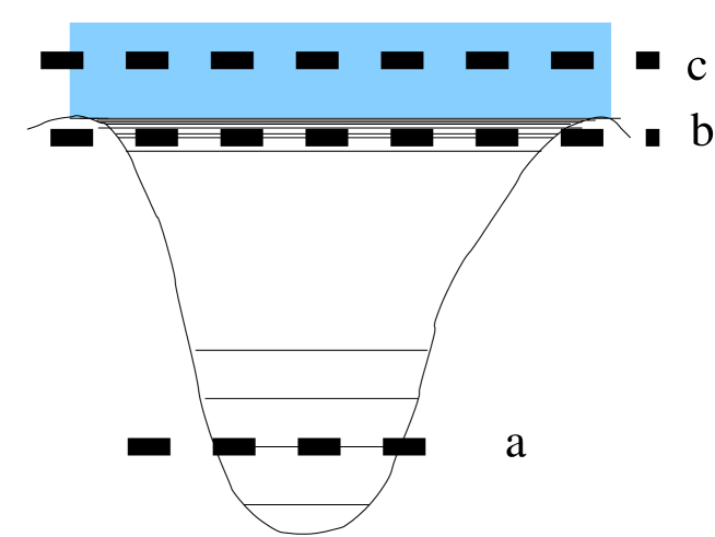
Figure 1: In the energy range “a” the system is unlikely to be ergodic. In “c” it is very likely ergodic, and in “b” it is almost ergodic. The width of the dashed line represents $\Delta E$

If the energy of the system described by the Hamiltonian for relative motion is in the region shown by the dashed line marked “a”, where $\delta_{i}$ is fairly large compared to $\Delta E$ we do not expect ergodic behaviour. We expect that if we start the molecule off in a pure state, such as the ground state or first excited state, it will remain there. This follows from purely energetic considerations.

The region marked “c” is a continuum where the molecule has dissociated and we have atomic Hydrogen. In this region $\delta_{i}\approx 0<<\Delta E$ and one expects ergodicity.

Region marked “b” is in between, with $\delta_{i}\approx\Delta E$ and one can expect ergodicity if the off diagonal matrix elements are large compared to $\delta_{i}$. As long as there are soft quanta that can be absorbed or emitted whose energies match the energy spacings ($\delta_{i}$), this will be the case. The soft quanta are provided by the inelastic collisions with other molecules. We thus expect that even if we start the system off in a pure state it will soon make transitions to the numerous other states in that energy band and be effectively described by a microcanonical density matrix. This is what we would like to demonstrate in Sections 4,5 and 6.

As the above example illustrates, the centre of mass degrees in a gas, for instance, typically are expected to be ergodic. They correspond to the $\delta_{i}=0$ case. Classical analysis of “billiard balls” in certain situation shows ergodicity even with a small number of balls [5]. We need not expect the quantum behaviour of this weakly interacting system to be very different.

The difficult question concerns the non-center-of-mass degrees that have non-zero $\delta_{i}$. Are they ergodic or not? It can happen sometimes that while the center-of-mass degrees are ergodic, the non-center-of-mass degrees are in a pure state. The point we are trying to make is that the value of the energy spacing $\delta_{i}$, is a crucial factor in deciding the answer.

2.6.2 QCD Plasma

Another example is that of heavy ion collision producing quark gluon plasma Clearly when the energy of collision is smaller than the energy gap in QCD the hadrons are still usefully described by wave functions. Once this gap is exceeded one can expect thermalisation. What are the soft quanta here? Presumably these are soft gluons. There are some points of similarity between this system and the hydrogen molecule example discussed above. Deconfinement here, presumably corresponds to the dissociation of the molecule there.

2.6.3 Sodium Vapour

Let us take another example, where again we expect to see two different kinds of ergodicity. As it turns out this example has some similarity with the black hole situation to be discussed later. Consider a vapour of sodium atoms. The centre of mass motion of the atoms is “gap-less” and can be expected to be ergodic motion, even at low temperatures. The electrons in the atom however are described by pure state wave functions, at temperatures that are low compared to electronic level spacings. Consider what happens when the vapour cools down sufficiently that it forms a Sodium crystal, at some low temperature. The centre of mass motion is no longer ergodic. However sodium being a metal, the outer electrons are free to move around in the crystal. They are now described by a Fermi gas and their motion is ergodic! One can presumably associate a temperature with them. The gap $\delta_{i}$ between electronic levels has changed from, say, a few electron volts to something of the order $1\over L$ where $L$ is the macroscopic size of the crystal. This is a quantum mechanical effect. Thus a phase transition in the material has introduced new gap-less excitations that demonstrate ergodic behaviour, even though at a higher temperature they were not ergodic (because they were confined to the interior of the sodium atom)!

2.6.4 Stars and Black Holes

There is a similarity between the sodium vapour example and the black hole example. When matter collapses to form a star the centre of mass motion of the lumps of matter once again can be assumed to be ergodic and as a consequence we get a hot star. (Indeed astrophysicists routinely treat this motion entirely classically using classical statistical mechanics, until we get to high densities.) At some point the star (if sufficiently massive) cools to essentially zero temperature, undergoes a phase transition and forms a black hole. At this point some other internal degrees of freedom (D-branes in string theory black holes) become (presumably gap-less and) ergodic and there is a temperature that can be associated with them. These are like the outer electrons of the sodium atom.

2.7 Summary

Let us summarize the points made in this section:

1. Coarse graining is done by introducing soft quanta $a$ in addition to the conventional microscopic degrees $i$. These soft modes induce transitions between the $|i\rangle$. The gap $\delta_{a}$ must be very small compared to the inverse time of observation. Also the off diagonal terms in the Hamiltonian connecting different $i$ states must be much larger than the unperturbed gap $\delta_{i}$. This is necessary for the exact energy eigenstates to satisfy the properties assumed in Section 3. This is thus necessary for ergodicity. In the resonance picture this will automatically be the case if there is a sufficient number of soft quanta with a continuum of frequencies in the appropriate energy range.

2. The interaction with the continuum $a$ degrees of freedom, induces an anti-Hermitean part to the effective Hamiltonian of the $i$ system. This makes the evolution look irreversible. The apparent lack of reversibility has to do with treating the $a$-degrees as continuous. If a gap $\delta_{a}$ is introduced, the recurrence time is $O({1\over\delta_{a}})$.

In section 6 we will calculate, in a simplified model, the time evolution of the partially traced density matrix that describes the $i$ system and show how it appears to evolve in time to a thermal one.

3 Mathematical Formulation of the Problem and Earlier Approaches

In this section we give a mathematical formulation of the problem we wish to address in this paper. It is helpful to start with a brief recapitulation of the situation in classical statistical mechanics. In particular we shall follow the Gibbsian route formulated on the classical phase space and even there we will be concerned only with the microcanonical ensemble description.

In such a situation one considers an isolated system with its total energy in a narrow band $E_{0}-\Delta<E<E_{0}+\Delta$. Under time evolution governed by the dynamical equations the system moves on this hyper-surface of the $6N$-dimensional phase space called the ”energy surface”. Different regions of this energy surface can be labeled by values of observables other than the Hamiltonian. Generically these observables are time-dependent. Further, the accuracies with which these observables can be determined make it meaningful to decompose the energy surface into elementary cells called ”phase cells” and all system points within the same cell are ascribed the same value for the ”coarse grained” observables Due to dynamics the system point moves from phase space cell to phase space cell.The crux of the Gibbsian statistical mechanics is the so called ergodic theorem( more precisely the quasi-ergodic theorem) which states that after a sufficiently long time the system point passes through all the phase cells and furthermore the time spent in each phase cell is proportional to its volume. This immediately allows one to equate the time average of observables with an ”ensemble average” wherein the weight factor for each phase cell is its volume. As the phase cells can be constructed with equal volume the ensemble average can be taken with a distribution giving equal weights to the different phase cells. This is the microcanonical distribution. The crucial point is that the time average has been replaced by an ensemble average in such a way that the distribution is independent of the initial state. It should be emphasized that in addition to the quasi-ergodic theorem one also approaches the same problem through the so called H-theorem and the concomitant concept of entropy.In what follows we shall only concentrate on the quasi-ergodic aspects of the problem.

Having stated all this it is very important to emphasize that a precise proof of the quasi-ergodic theorem and in particular the resolution of the precise role of dynamics is a very difficult problem. Both in this formulation as well as in the Boltzmannian approach to statistical mechanics assumptions have to be made that are equivalent to the assumption of chaotic behaviour.

3.1 Formulation of Quantum Statistical Mechanics.

Now the main question is how to formulate and prove similar statements in the context of quantum mechanics. The foremost difficulty here is that unlike as in classical mechanics there is no concept of a phase space nor of a trajectory.If classically one views the phase space as the space of all possible states of the classical system, the natural analog in the quantum case is the Hilbert space. Already at this stage many crucial differences appear; one such is the fact that for even a simple system like the ideal gas while the classical phase space is finite-dimensional with dimension $6N$, the quantum mechanical Hilbert space ${\cal H}$ is the tensor product of $N$ copies of Hilbert spaces ${\cal H}_{i}$ each of which is infinite-dimensional.

Let $H$ be the exact Hamiltonian of the system and let $|A\rangle$ be the exact eigenstate with eigenvalue $E_{A}$. Now Consider energy eigenstates such that their eigenvalues are in the range $E_{0}-\Delta<E_{A}<E_{0}+\Delta$. Further, let the initial state of the system $|\psi\rangle$ be such that

$$|\psi\rangle=\sum_{A}C_{A}^{\psi}|A\rangle$$ (3.1.1)

Then

$$|\psi(t)\rangle=\sum_{A}~{}C_{A}^{\psi}~{}e^{-iE_{A}t}~{}|A\rangle$$ (3.1.2)

If we denote $C_{A}^{\psi}(t)=C_{A}^{\psi}e^{-iE_{A}t}$ it is obvious that $|C_{A}(t)|^{2}$ are independent of time for all A. The average energy of the system at any time t is given by

$$\bar{E}(t)=\sum_{A}|C_{A}(t)|^{2}E_{A}$$ (3.1.3)

¿From eqn (3.1.3) we see another principal difference between the classical and quantum situations: in the quantum case not only is $\bar{E}$ constant in time, but so are all the quantities $|C_{A}|^{2}$. If we now decompose $C_{A}(t)$ into its magnitude $r_{A}$ and its phase $\theta_{A}$ we find that while $r_{A}$ does not change with time, $\theta_{A}(t)=\theta_{A}(0)-E_{A}t$.

¿From this it follows that under quantum dynamics i.e Schrőedinger equation, the motion of the system point is not over the entire Hilbert space but over the subspace defined by constant $|C_{A}(t)|^{2}$ for each $A$. The motion is in fact on the $N_{A}$-torus spanned by the angle variables $\theta_{A}$ where $N_{A}$ is the number of (non-degenerate)energy eigenvalues in the interval considered. Furthermore, the motion on this $N_{A}$-torus is such that the angular velocity ${d\theta(t)\over dt}$ is constant in every direction and equal to $-E_{A}$. For a macroscopic system the Hamiltonian $H$ will be generically so complex that this motion will densely fill the entire $N_{A}$-torus and because of the uniform velocity in every direction the time spent by the system point in any interval $[\{\theta_{A}\},\{\theta_{A}+\delta\theta_{A}\}]$ is exactly proportional to the volume of the interval. In this sense the quantum motion is quasi-ergodic. The precise conditions to be fulfilled by the spectrum of eigenvalues of $H$ will be discussed later but it suffices to stress here that they are fairly generic and unlike the classical case do not require special assumptions about chaos. Now consider the expectation value of an observable $O$ in the state $|\psi(t)\rangle$:

$$\langle\psi(t)|O|\psi(t)\rangle=\sum_{A,B}~{}C_{B}^{*\psi}~{}C_{A}^{\psi}~{}e^{-i(E_{A}-E_{B})t}~{}~{}O_{BA}$$ (3.1.4)

and a time-average of this expectation value over a duration $T$ centred at time $\tau$

$$\bar{O}(\tau) = {1\over 2T}~{}\int_{\tau-T}^{\tau+T}~{}~{}\langle\psi(t)|A|\psi(t)\rangle$$ (3.1.5)

$$= \sum_{B,A}C_{B}^{*\psi}~{}C_{A}~{}O_{BA}~{}e^{-i(E_{A}-E_{B})\tau}{\sin{(E_{A}-E_{B})T}\over(E_{A}-E_{B})T}$$

Now the main problem is that this expression has an explicit dependence on the parameters $C_{A}^{\psi}$ of the initial state and can not be replaced by an ensemble average that is insensitive to the initial state. This is the mathematical formulation of the problem to be solved i.e interpret quantum statistical mechanics in such a way that the time-average does not remember the initial state.

It is necessary to make more precise the notion of the time-average. Note that

$${\sin(ET)\over(ET)}_{T\rightarrow\infty}\rightarrow\delta(E)$$ (3.1.6)

The time average in eqn (3.1.5) then becomes

$$\bar{O}(\tau)=\sum_{A}|C_{A}^{\psi}|^{2}O_{AA}.$$ (3.1.7)

At this stage nothing more can be said. If we however consider some special class of systems it is possible to make more statements. For example, Berry [32] has conjectured that for classically chaotic systems energy eigenfunctions behave like Gaussian random variables. More precisely consider expanding the exact energy eigenstates $|A\rangle$ in some orthonormal basis $|I\rangle$

$$|A\rangle=\sum_{I}C_{A}^{I}|I\rangle$$ (3.1.8)

Then the Berry conjecture amounts to saying that $C_{A}^{I}$ are independently distributed random numbers. At this stage it is sufficient to just specify the two-point correlation of this distribution

$$\langle C_{A}^{*I}C_{B}^{J}\rangle_{ens}={1\over N_{A}}\delta_{AB}\delta_{IJ}$$ (3.1.9)

It is easy to see that eqn (3.1.9) is compatible with unitarity. Despite the apparent basis dependence of this criterion, it is actually basis independent.To see this let us expand $|A\rangle$ in another orthonormal basis $I^{\prime}$

$$|A\rangle=\sum_{I}^{\prime}C_{A}^{I^{\prime}}|I^{\prime}\rangle$$ (3.1.10)

with

$$|I^{\prime}\rangle=B^{I^{\prime}}_{I}|I\rangle$$ (3.1.11)

Then

$$C_{A}^{I^{\prime}}=\sum_{I}B_{I}^{I^{\prime}}C_{A}^{I}$$ (3.1.12)

and

$$\langle C_{A}^{*I^{\prime}}C_{B}^{I^{\prime}}\rangle_{ens} = \sum_{IJ}B_{I}^{*I^{\prime}}B_{J}^{J^{\prime}}\langle C_{A}^{*I}C_{B}^{J}\rangle_{ens}$$ (3.1.13)

$$= {1\over N_{A}}\sum_{IJ}B_{I}^{*I^{\prime}}B_{J}^{J^{\prime}}\delta_{AB}\delta_{IJ}$$

$$= {1\over N_{A}}\delta_{AB}\delta_{I^{\prime}J^{\prime}}$$

where we have made use of the unitarity of the transformation matrix $B_{I}^{I^{\prime}}$. It should be noted that this proof works only when the bases ${I},{I^{\prime}}$ etc. are not derived from the energy basis by application of fixed unitary transformations on the energy-eigenfunction basis. Now let us consider the ensemble-average of eqn (3.1.7):

$$\langle\sum_{A}|C_{A}^{\psi}|^{2}O_{AA}\rangle_{ens} = \sum_{AIJ}|C_{A}^{\psi}|^{2}\langle C_{A}^{*I}C_{A}^{J}\rangle_{ens}O_{IJ}$$ (3.1.14)

$$= {1\over N_{A}}\sum_{AIJ}|C_{A}^{\psi}|^{2}\delta_{IJ}O_{IJ}$$

$$= {1\over N_{A}}\sum_{A}|C_{A}^{\psi}|^{2}\sum_{I}O_{II}$$

$$= {1\over N_{A}}\sum_{I}O_{II}$$

Let us also consider the average of $O$ at a particular instant given by eqn (3.1.4):

$$\langle\sum_{AB}C_{B}^{*\psi}C_{A}^{\psi}e^{-i(E_{A}-E_{B})t}O_{BA}\rangle_{ens} = \sum_{ABIJ}C_{B}^{*\psi}C_{A}^{\psi}\langle C_{A}^{*I}C_{B}^{J}\rangle_{ens}O_{IJ}e^{-i(E_{A}-E_{B})t}$$ (3.1.15)

$$= {1\over N_{A}}\sum_{ABIJ}C_{B}^{*\psi}C_{A}^{\psi}\delta_{AB}\delta_{IJ}e^{-i(E_{A}-E_{B})t}O_{IJ}$$

$$= {1\over N_{A}}\sum_{AI}C_{A}^{*\psi}C_{A}^{\psi}O_{II}$$

$$= {1\over N_{A}}\sum_{I}O_{II}$$

which is the same as eqn (3.1.14). Thus in these cases the time-average is equal to the value at any given instant of time once the ensemble average is taken and in both of them all memory of the initial state is lost. The drawback with this picture is that the equality seems to hold at arbitrary times $t$ while one should only expect it at late times. In other words there is no way to understand ”thermalization times” in this picture.

For eqn (3.1.6) to hold it actually suffices for $T>>{1\over\delta}$ where $\delta$ is the spacing between the exact energy eigenvalues. As this spacing typically decreases exponentially with the size of the system the corresponding $T$ is exponentially large in system size. This is analogous to the classical case where for very very large times the Poincare recurrence theorem [8, 9] guarantees the equality of time and ensemble averages.

Clearly what’s important are not such astronomically large time-scales. Instead, consider the more moderate and intermediate time-scale
${1\over\Delta}~{}<T~{}<<{1\over\delta}$: then one has

$${\sin(E_{m}-E_{n})T\over(E_{m}-E_{n})T}\simeq 1$$

and consequently

$$\bar{O}(\tau)=\sum C^{*\psi}_{B}~{}C^{\psi}_{A}~{}~{}e^{-i(E_{A}-E_{B})\tau}A_{BA}$$ (3.1.16)

Again if the spectrum of the Hamiltonian is sufficiently complex and there are no degeneracies, for any reasonable value of $\tau$ there will be cancelations among all the $A\neq B$ terms and one again gets back to eqn (3.1.7). Actually for such complex systems even the average at any particular instant(except for pathologically small values of $\tau$) becomes the same as eqn (3.1.7) and one does not even need to do any time averaging. But eqn (3.1.7) retains memory of the initial state and at this stage it is not possible to recover the basis of statistical mechanics unless one postulates additional assumptions like Berry’s conjecture etc. (we will show later ways of going beyond such restrictive assumptions; that will be the main result of this paper).

In [31] there was a proposal to consider a different approach to this problem by assuming that observables of interest are of the type:

$$O_{BA}~{}=~{}O_{0}~{}\delta_{BA}~{}~{}+R_{BA}$$ (3.1.17)

with $R_{BA}$ being ”small”.

Now too $\langle\psi(t)|O|\psi(t)\rangle$ is of the same form as eqn(3.1.7) except for small corrections due to the $R_{BA}$ terms. Once again if we interpret this restriction in the Schrődinger picture one would get eqn (3.1.7) to be true at all times which does not make much sense. A possibility is to interpret $\langle\psi(t)|O|\psi(t)\rangle$ as $\langle\psi|O(t)|\psi\rangle$ in the Heisenberg picture and assume eqn (3.1.17) only for late times. Even then one has to still introduce some ”ensemble average” along the lines of Berry’s conjecture and there seems to be no scope for addressing the issue of ”thermalization time” at all. We will see later that eqn (3.1.17) is too strong a restriction on macroscopic observables and in fact implies that in the classical limit these observables are constant on the entire energy surface.

3.2 Earlier approaches

Much after we had finished our work( to be described in detail in secs 4, 5 and 6) we came to know of the fundamental paper on this subject due to J. von Neumann [10] through ref [22]. Subsequently we have traced Pauli and Fierz’s [11] sequel to von Neumann’s work as well as Van Kampen’s formulation [12] of the problem. There are differences between von Neumann’s and Van Kampen’s approaches but they are essentially similar in spirit and both give a quantum mechanical equivalent of the classical phase space cell decomposition. While von Neumann uses fairly rigorous methods to show that the time average of the expectation values of the macroscopic observables (defined suitably by him) approaches arbitrarily closely the microcanonical average( he also shows that a suitably defined entropy, different from what is known as von Neumann entropy in the literature, also approaches the entropy of the microcanonical distribution which is the quantum version of the H-theorem). Van Kampen establishes a master equation for the probability distribution for finding the system in various phase cells given the distribution at $t=0$ and argues that it has all the properties of a Markov process whence the problem becomes identical to the one in classical statistical mechanics. While in von Neumann’s treatment the issue of thermalization time is not very transparent, in Van Kampen’s treatment it can be handled in principle exactly as in classical statistical mechanics.

While the mathematical formalism in all three approaches have strong overlaps, our treatment is rather different in its interpretation of coarse graining in quantum mechanics which is somewhat kinematical in origin in both von Neumann’s and Van Kampen’s treatments. We seek a dynamical origin for this coarse-graining. In our approach, the extra soft quanta not only play a passive role as the degrees that are coarse grained away, they directly provide the mechanism for thermalization. Thermalization takes place due to emission and absorption of these soft quanta. Furthermore in order for this thermalization to happen it is crucial that they have the properties described in Sec 2.4 and 2.5. Thus the reader will see that the setup of Section 4, where the solution to the problem of ergodicity is given in an abstract way is, perhaps not surprisingly, mathematically identical to the setup of von Neumann. Both of them describe a quantum mechanical analogue of Gibbsian coarse graining. Section 5 and Section 6 where the soft quanta play out their role in thermalization have, no obvious counterpart in von Neumann’s discussion.

We include a short description of the works of von Neumann and van Kampen for reasons of completeness and historical accuracy. This should also provide a perspective for the whole discussion. This section is not a prerequisite for understanding the rest of this paper. For convenience we have given at appropriate places below our notation used in Section 4 corresponding to each of von Neumann’s symbols.

3.2.1 Quantum Statistical Mechanics of von Neumann

The three essential ingredients of this approach are i)energy-surfaces,ii)phase cells belonging to a particular energy surface and iii)micro-states spanning each phase cell.

Energy Surfaces:The exact Hamiltonian of the system is taken to be $H$ whose spectrum is assumed to be discrete for simplicity.If $\Delta E$ is the macroscopic resolution with which energy measurements can be made, the energy levels are divided into groups of width $\Delta E$ each and the groups are labeled by $a=1,2,...$. This means that only energy levels belonging to different groups are macroscopically distinct.The energy eigenvalues are labeled $W_{\rho,a}$ with $\rho=1,2,...,S_{a}$. (In Section 4 we have used $A$ to label the exact energy eigenstates. $S_{a}$ corresponds to $N_{A}$ of Section 4, where we have restricted ourselves to one energy surface.) The eigenfunctions are labeled $\phi_{\rho,a}$. Thus $S_{a}$ is the number of microscopic states spanning the energy surface $a$. The projection operator corresponding to $\phi_{\rho,a}$ is denoted by ${\bf P}_{\phi_{\rho,a}}$.

Macroscopic Observables: von Neumann considers all macroscopic observations to be simultaneous and therefore all macroscopic observables to be mutually commuting. (The word “macroscopic” is used here in the sense of Quantum Measurement Theory. It does not mean macroscopic in the sense of statistical mechanics (i.e. pressure, density, etc ). Indeed they correspond to micro-state variables such as the position coordinates of molecules of a gas except that macroscopic measurements can not resolve their values within a phase cell. These observables are thus a subset of the $O$ of Section 4). Their simultaneous eigenfunctions are denoted by $\omega_{\lambda,p},\lambda=1,2,..,s_{p}$ where distinct values of $p$ denote distinct values of the observables but all states with the same $p$ but different $\lambda$ have the same values for all observables. (In Section 4 we have used ‘$a$‘ for $\lambda$, and ‘$i$‘ for $p$. $s_{p}$ is $N_{a}$ of Section 4. The simultaneous eigenstates there are denoted by $|i,a\rangle$.)

The projection operator for the state $\omega_{\lambda,p}$ is denoted by ${\bf P}_{\phi_{\lambda,p}}$ and the density matrix signifying an equal mixture of $\omega_{\lambda,p}$ for the same $p$ but for all possible values of $\lambda$ is denoted by

$${1\over s_{p}}{\bf E}_{p}\equiv\sum^{s_{p}}_{\lambda}{\bf P}_{\omega_{\lambda,p}}$$ (3.2.18)

Eqn (3.2.18) can be taken as the density matrix for a ”phase space cell”. In von Neumann’s paper the explicit construction of these mutually commuting macroscopic observables is not given and the discussion not very transparent. Van Kampen treats this in a more transparent manner. Consider any observable $O$ and express it in the exact energy-eigenfunction basis

$$O=\sum_{\rho,a,\sigma,b}O_{\rho,a;\sigma,b}|\phi_{\rho,a}\rangle\langle\phi_{\sigma,b}|$$ (3.2.19)

Van Kampen argues that the matrix elements of the time-dependent operator $O(t)$

$$O(t)_{\rho,a,\sigma,b}=O_{\rho,a,\sigma,b}e^{-i(W_{\rho,a}-W_{\sigma,b})}$$ (3.2.20)

are associated with very rapid fluctuations whenever $a\neq b$.Thus it makes sense to replace the microscopic operator $O$ by

$$O^{\prime}=\sum_{\rho,a,\sigma,a}O_{\rho,a;\sigma,a}|\phi_{\rho,a}\rangle\langle\phi_{\sigma,a}|$$ (3.2.21)

Equivalently

$$O^{\prime}_{\rho,a;\sigma,b}=O_{\rho,a;\sigma,a}~{}\delta_{ab}$$ (3.2.22)

Van Kampen also introduces the coarse-grained energy operator to be

$$H^{\prime}=\sum_{a}W_{a}\sum_{\rho}^{S_{a}}{\bf P}_{\phi_{\rho,a}}$$ (3.2.23)

Note that all the energy eigenvalues belonging to an energy-surface have been replaced by a single value $W_{a}$. Now it is easy to see that $H^{\prime},O^{\prime}$ commute so they can be simultaneously diagonalised:

$$H^{\prime}|\omega_{\mu,a}\rangle = W_{a}|\omega_{\mu,a}\rangle$$

$$O^{\prime}|\omega_{\mu,a}\rangle = A_{\mu,a}|\omega_{\mu,a}\rangle$$ (3.2.24)

He now introduces the coarse-grained observables by grouping the eigenvalues $A_{\mu,a}$ into phase cells in such a way that only those belonging to different groups(cells) can be distinguished macroscopically i.e through macroscopic measurements.Let these groupings be labeled by $\nu=1,2,...N_{a}$ ($N_{a}$ of von Neumann is $N_{i}$ of Section 4). Then

$${\tilde{O}}=\sum_{a}\sum_{\nu}A_{\nu,a}\sum_{\lambda}^{s_{\nu,a}}{\bf P}_{\omega_{\lambda,\nu,a}}$$ (3.2.25)

Now it is clear that all such macroscopic observables commute with each other with $\omega_{\lambda,\nu,a}$ as their simultaneous eigenfunctions. Furthermore,in this approach, the phase cells, labeled by $\nu,a$ are neatly partitioned into disjoint sets by the energy surfaces.

It is instructive to compare this construction with von Neumann’s treatment( and later with ours). von Neumann argues that any operator with a boolean spectrum( eigenvalues $0$ or $1$) is a macroscopic observable and every macroscopic observable has a spectral decomposition of the type

$$A=\sum_{p}c_{p}{\bf E}_{p}$$ (3.2.26)

He then considers the function $f_{a}(x)$ such that $f_{a}=1$ if $x$ belongs to the energy eigenvalues of the energy surface labeled by $a$ and $0$ otherwise. Then the operator $f_{a}(H)$ has eigenvalues $0,1$ and is thus a macroscopic observable. By eqn(3.2.26) it must admit the decomposition

$$f_{a}(H)=\sum_{p}f_{a}^{p}{\bf E}_{p}$$ (3.2.27)

On the other hand

$$f_{a}(H)=\sum_{\rho=1}^{S_{a}}{\bf P}_{\phi_{\rho,a}}$$ (3.2.28)

As both $f_{a}(H)$ and ${\bf E}_{p}$ for every p are equal to their own squares and as the product of two distinct ${\bf E}_{p}$’s is zero, it follows that ${f_{a}^{p}}^{2}={f_{a}^{p}}$ for every $p$ i.e $f_{a}^{p}$ is either $1$ or $0$. Relabeling all those $p$’s for which$f_{a}^{p}=1$ by $\nu,a$ we have

$$\sum_{\rho}^{S_{a}}{\bf P}_{\phi_{\rho,a}}=\sum_{\nu}^{N_{a}}{\bf E}_{\nu,a}$$ (3.2.29)

i.e we again have a unique partitioning of all the phase cells among the energy surfaces. The equivalent of this in our approach is given by the construction in sec. 4.1.

Microcanonical ensemble:
We briefly sketch JvN’s proof showing the asymptotic equivalence of the time averaged expectation value and the microcanonical average. We denote the operator occurring in eqn (3.2.29) by $\Delta_{a}$. It is then clear that ${1\over S_{a}}\Delta_{a}$ is the density matrix for an equal mixture of energy eigenstates belonging to the energy surface $a$ and as such represents the density matrix for the microcanonical ensemble associated with that energy surface. If the initial state $\psi$ is such that $(\Delta_{a}\psi,\psi)$ is nonzero for several values of $a$, one should consider a mixture of microcanonical ensembles for each $a$ with weight factor $(\Delta_{a}\psi,\psi)$(this is the probability of finding the system in the energy surface $a$). Thus the microcanonical density matrix in the general case is

$$U_{\psi}=\sum_{a=1}^{\infty}{(\Delta_{a}\psi,\psi)\over S_{a}}\Delta_{a}$$ (3.2.30)

In our treatment later on we shall consider only one energy surface.

Quantum Ergodicity

Next JvN considers the system to be initially in a state

$$|\psi\rangle=\sum_{a=1}^{\infty}\sum_{\rho=1}^{S_{a}}r_{\rho,a}e^{i\alpha_{\rho,a}}|\phi_{\rho,a}\rangle~{}~{}~{}~{}(r_{\rho,a}\geq 0,0\leq\alpha_{\rho,a}<2\pi)$$ (3.2.31)

then

$$|\psi(t)\rangle=\sum_{a=1}^{\infty}\sum_{\rho=1}^{S_{a}}r_{\rho,a}e^{-i({2\pi\over h}W_{\rho,a}t-\alpha_{\rho,a})}$$ (3.2.32)

Introducing the abbreviations

$$x_{\nu,a}=({\bf E}_{\nu,a}\psi(t),\psi(t))~{}~{}~{}~{}u_{a}=(\Delta_{a}\psi(t),\psi(t))=(\Delta_{a}\psi,\psi)$$ (3.2.33)

one considers a macroscopic observable $A$

$$A=\sum_{a=1}^{\infty}\sum_{\nu=1}^{N_{a}}~{}\eta_{\nu,a}{\bf E}_{\nu,a}$$ (3.2.34)

The expectation value of $A$ in the state $\psi(t)$ is then

$$E_{A}(\psi(t))=(A\psi(t),\psi(t))=\sum_{a=1}^{\infty}\sum_{\nu=1}^{N_{a}}\eta_{\nu,a}({\bf E}_{\nu,a}\psi(t),\psi(t))=\sum_{a=1}^{\infty}\sum_{\nu=N_{a}}\eta_{\nu,a}x_{\nu,a}$$ (3.2.35)

while the microcanonical average is

$$E_{A}(U_{\psi})=TrAU_{\psi} = Tr(\sum_{a=1}^{\infty}\sum_{\nu=1}^{N_{a}}\eta_{\nu,a}{\bf E}_{\nu,a}\sum_{a^{\prime}=1}^{\infty}\sum_{\nu^{\prime}=1}^{N_{a^{\prime}}}{u_{a^{\prime}}\over S_{a^{\prime}}}{\bf E}_{\nu^{\prime},a^{\prime}})$$ (3.2.36)

$$= \sum_{a=1}^{\infty}\sum_{\nu=1}^{N_{a}}\eta_{\nu,a}{u_{a}s_{\nu,a}\over S_{a}}$$

On using the eqn (3.2.36) and Schwarz’s inequality JvN finally obtains

$$(E_{A}(\psi(t))-E_{A}(U_{\psi}))^{2}\leq{\bar{\eta}}^{2}\sum_{a=1}^{\infty}\sum_{\nu=1}^{N_{a}}{S_{a}\over s_{\nu,a}u_{a}}[x_{\nu,a}-{s_{\nu,a}u_{a}\over S_{a}}]^{2}$$ (3.2.37)

where

$${\bar{\eta}}^{2}=\sum_{a=1}^{\infty}\sum_{\nu=1}^{N_{a}}{s_{\nu,a}u_{a}\over S_{a}}\eta_{\nu,a}$$ (3.2.38)

JvN finally establishes that the time average of the lhs of eqn (3.2.37) is bounded by ${\bar{\eta}}^{2}max_{a}\{{2N_{a}\over S_{a}}\}$.

3.2.2 Van Kampen’s approach

Van Kampen expands the initial state $\psi$ not in terms of the exact eigenfunctions of the Hamiltonian but in terms of the simultaneous eigenstates $\omega_{\lambda,\nu,a}$ of the coarse grained observables( we are retaining the notation of JvN):

$$|\psi\rangle=\sum_{\lambda,\nu,a}b_{\lambda,\nu,a}|\omega_{\lambda,\nu,a}\rangle$$ (3.2.39)

The probability of finding the system in the phase cell $\nu,a$ is given by

$$P_{\nu,a}=\sum_{\lambda=1}^{s_{\nu,a}}|b_{\lambda,\nu,a}|^{2}$$ (3.2.40)

The time dependence of the state is given by

$$|\psi(t)\rangle=\sum_{\lambda,\nu,a}b_{\lambda,\nu,a}(t)|\omega_{\lambda,\nu,a}\rangle$$ (3.2.41)

where

$$b_{\lambda,\nu,a}(t)=\sum_{\lambda^{\prime},\nu^{\prime},a^{\prime}}\langle\omega_{\lambda,\nu,a}|U(t)|\omega_{\lambda^{\prime},\nu^{\prime},a^{\prime}}\rangle$$ (3.2.42)

and $U(t)$ is the time-evolution operator. The probability of finding the system in the phase cell $\nu,a$ at time $t$ is given by

$$P_{\nu,a}(t)=\sum_{\stackrel{{\scriptstyle\lambda^{\prime},\nu^{\prime},a^{\prime}}}{{\lambda^{\prime\prime},\nu^{\prime\prime},a^{\prime\prime}}}}\sum_{\lambda}\langle\omega_{\lambda,\nu,a}|U(t)|\omega_{\lambda^{\prime},\nu^{\prime},a^{\prime}}\rangle\langle\omega_{\lambda,\nu,a}|U(t)|\omega_{\lambda^{\prime\prime},\nu^{\prime\prime},a^{\prime\prime}}\rangle^{*}b_{\lambda^{\prime},\nu^{\prime},a^{\prime}}(0)b^{*}_{\lambda^{\prime\prime},\nu^{\prime\prime},a^{\prime\prime}}(0)$$ (3.2.43)

Invoking the argument that the summation consists of many wildly fluctuating terms and all the non-negative terms cancel i.e only surviving terms are ${\nu^{\prime},a^{\prime}}={\nu^{\prime\prime},a^{\prime\prime}}$ and $\lambda^{\prime}=\lambda^{\prime\prime}$.This reduces eqn(3.2.41) to

$$P_{\nu,a}(t)=\sum_{\nu^{\prime},a^{\prime}}\sum_{\lambda^{\prime}}\sum_{\lambda}|\langle\omega_{\lambda,\nu,a}|U(t)|\omega_{\lambda^{\prime},\nu^{\prime},a^{\prime}}\rangle|^{2}|b_{\lambda^{\prime},\nu^{\prime},a^{\prime}}(0)|^{2}$$ (3.2.44)

Van Kampen further argues that in a sum of type

$$\sum_{i}\alpha_{i}\beta_{i}$$

where both $\alpha_{i},\beta_{i}$ are rapidly fluctuating but positive it is a good approximation to evaluate the sum as

$${1\over G}\sum_{i}\alpha_{i}\sum_{i}\beta_{i}$$

With this approximation eqn (3.2.44) becomes

$$P_{\nu,a}(t)=\sum_{\nu^{\prime},a^{\prime}}{1\over s_{\nu,a}}\sum_{\lambda,\lambda^{\prime}}|\langle\omega_{\lambda,\nu,a}|U(t)|\omega_{\lambda^{\prime},\nu^{\prime},a^{\prime}}\rangle|^{2}P_{\nu^{\prime},a^{\prime}}(0)$$ (3.2.45)

With the definition

$$T_{t}(\nu,a|\nu^{\prime},a^{\prime}){\stackrel{{\scriptstyle def}}{{=}}}{1\over s_{\nu,a}}\sum_{\lambda,\lambda^{\prime}}|\langle\omega_{\lambda,\nu,a}|U(t)|\omega_{\lambda^{\prime},\nu^{\prime},a^{\prime}}\rangle|^{2}$$ (3.2.46)

eqn (3.2.45) can be recast as

$$P_{\nu,a}(t)=\sum_{\nu^{\prime},a^{\prime}}T_{t}(\nu,a|\nu^{\prime},a^{\prime})P_{\nu^{\prime},a^{\prime}}(0)$$ (3.2.47)

As there is nothing special about the instant $t=0$ it follows that

$$P_{\nu,a}(t_{1}+t_{2})=\sum_{\nu^{\prime},a^{\prime}}T_{t_{2}}(\nu,a|\nu^{\prime},a^{\prime})P_{\nu^{\prime},a^{\prime}}(t_{1})$$ (3.2.48)

Equivalently

$$T_{t_{1}+t_{2}}(\nu,a|\nu^{\prime},a^{\prime})=\sum_{\nu^{\prime\prime},a^{\prime\prime}}T_{t_{2}}(\nu,a|\nu^{\prime\prime},a^{\prime\prime})T_{t_{1}}(\nu^{\prime\prime},a^{\prime\prime}|\nu^{\prime},a^{\prime})$$ (3.2.49)

Along with the obvious properties of $T_{t}(\nu,a|\nu^{\prime},a^{\prime})$

$$T_{0}(\nu,a|\nu^{\prime},a^{\prime})=\delta_{\nu,a;\nu^{\prime},a^{\prime}};~{}~{}~{}T_{t}(\nu,a|\nu^{\prime},a^{\prime})\geq 0;~{}~{}~{}\sum_{\nu,a}T_{t}(\nu,a|\nu^{\prime},a^{\prime})=1$$ (3.2.50)

which follow from the orthogonality of $|\omega_{\lambda,\nu,a}\rangle,|\omega_{\mu,\nu^{\prime},a^{\prime}}\rangle$ for distinct $\{\nu,a\},\{\nu^{\prime},a^{\prime}\}$ and the unitarity of $U(t)$, one concludes that $T_{t}$ is a Markov Process. One knows from the Frobenius-Perron theorem that there is always an equilibrium distribution $P^{eq}_{\nu,a}$. From the spectrum of the operator $T(\nu,a|\nu^{\prime},a^{\prime})$ one can also deduce the thermalization times.

Before concluding this section it is instructive to derive the so called Master equation. For this one solves for $T_{\Delta t}$ as

$$T_{\Delta t}(\nu,a|\nu^{\prime},a^{\prime})=\delta_{\nu,a;\nu^{\prime},a^{\prime}}\{1-\Delta t\sum_{\nu^{\prime\prime},a^{\prime\prime}}W_{\nu^{\prime\prime},a^{\prime\prime};\nu,a}\}+\Delta tW_{\nu,a;\nu^{\prime},a^{\prime}}$$ (3.2.51)

Then one gets the differential form of the Chapman-Kolmogorov equation

$${\partial\over\partial t}T_{t}(\nu,a|\nu^{\prime},a^{\prime})=\sum_{\nu^{\prime\prime},a^{\prime\prime}}W_{\nu,a;\nu^{\prime\prime},a^{\prime\prime}}T_{t}(\nu^{\prime\prime},a^{\prime\prime}|\nu^{\prime},a^{\prime})-W_{\nu^{\prime\prime},a^{\prime\prime};\nu,a}T_{t}(\nu,a|\nu^{\prime},a")$$ (3.2.52)

This can be recast in terms of $P_{\nu,a}(t)$ as

$${d\over dt}P_{\nu,a}(t)=\sum_{\nu^{\prime},a^{\prime}}\{W_{\nu,a;\nu^{\prime},a^{\prime}}P_{\nu^{\prime},a^{\prime}}-W_{\nu^{\prime},a^{\prime};\nu,a}P_{\nu,a}(t)\}$$ (3.2.53)

which is the master equation.

4 Quantum coarse graining and emergence of the microcanonical ensemble.

As we have stated already the major conceptual problem in Quantum statistical mechanics is that of understanding how a quantum state initially described by a pure density matrix can ever resemble the state of thermodynamic equilibrium which is clearly described by a mixed density matrix.

4.1 Coarse graining

As was clearly stressed by Gibbs [7] long ago, coarse graining is essential to understanding even the most basic features of classical statistical mechanics. We now introduce our proposal for a quantum coarse graining and show subsequently that the microcanonical distribution then follows for a large class of systems.

We consider two types of mutually commuting variables $I,{\cal A}$ and their simultaneous eigenstates $|i,a\rangle$. Later on we will define $|i,a\rangle$ only in the subspace spanning the states relevant for the microcanonical ensemble. The $i$ will eventually correspond to the labels of the usual micro-states entering the description of the statistical system and the precise nature of $a$ are not specified at present. Alternately one can think of $|i,a\rangle$ as the labeling of micro-states on the fine scale and $|i\rangle$ as the labeling of the micro-states at the coarse grained level.

It is assumed that to a very good approximation the ${\cal A}$ variables couple weakly to the $I$-variables in the total Hamiltonian i.e

$$H_{tot}=H^{(i)}+H^{(a)}+\lambda~{}~{}H^{(i,a)}$$ (4.1.1)

with $\lambda$ very small. Let $|A^{*}\rangle$ be the eigenstates of $H^{(i)}$ that lie in the range $E_{0}-\Delta E<E_{0}+\Delta$. We then form the matrix $I^{*}_{AB}=\langle B^{*}|I|A^{*}\rangle$ which is $N_{i}\times N_{i}$. Now let $|i\rangle$ be the eigenstates of $I^{*}$ and let $|i,a\rangle=|i\rangle\otimes|a\rangle$ where $|a\rangle$ are the eigenstates of $\cal A$ and let us also assume that there are $N_{a}$ such states. (A special choice could be $I=H^{(i)}$, in which case $|i\rangle=|A^{*}\rangle$.)

The important point is that the $N_{i}\times N_{a}$ states $|i,a\rangle$ continue to form a basis in terms of which all the exact energy eigenstates in the microcanonical band can still be expanded. It is of course important to state that even a small perturbation characterized by $\lambda$ can completely alter the nature of the eigenstates of the Hamiltonian $H$ because of the exponential crowding of the ”unperturbed” states but the number of eigenstates remains unchanged. The parameters of the microcanonical band $E_{0},\Delta$ are also most likely affected by the perturbation, but as we shall never need their precise values it does not matter for the ensuing discussion.

We shall only consider those observables that are insensitive to the $a$ labels i.e $\langle i,a|O|j,b\rangle=O_{ij}\delta_{ab}$. This is in keeping with the spirit of coarse graining described in Section 2.2.

4.2 Some preliminaries

Consider some arbitrary state in the subspace we have considered

$$|\psi\rangle=\sum C^{\psi}_{A}|A\rangle$$ (4.2.2)

where now $|A\rangle$ are the exact energy eigenstates of the system. Further, let

$$|A\rangle=\sum_{i,a}~{}~{}C_{A}^{*ia}~{}~{}|i,a\rangle$$ (4.2.3)

with the inverse expansion

$$|i,a\rangle=\sum_{A}~{}~{}C^{ia}_{A}~{}~{}|A\rangle$$ (4.2.4)

The coefficients $C_{A}^{ia}$ satisfy the following unitarity conditions:

$$\sum_{A}C_{A}^{*ia}~{}C_{A}^{i^{\prime}a^{\prime}}=\delta_{ii^{\prime}}\delta_{aa^{\prime}}~{}~{}~{}~{}~{}~{}\sum_{ia}C_{A}^{ia}C_{A^{\prime}}^{*ia}=\delta_{AA^{\prime}}$$ (4.2.5)

In terms of these definitions we can rewrite

$$\langle\psi|O|\psi\rangle=\sum_{A,B}~{}~{}C^{*\psi}_{B}~{}~{}C^{\psi}_{A}~{}~{}\langle B|O|A\rangle$$ (4.2.6)

as

$$O_{\psi\psi}~{}~{}=~{}~{}\sum_{a,ij}~{}\sum_{A,B}~{}C^{*\psi}_{B}~{}~{}C^{\psi}_{A}~{}~{}C_{A}^{*ia}~{}C_{B}^{ja}O_{ij}$$ (4.2.7)

Now introduce

$$\sum_{a}C_{A}^{ja}C_{B}^{*ka}=~{}~{}\delta_{jk}~{}~{}\delta_{AB}~{}~{}P^{j}_{A}+R^{jk}_{AB}$$ (4.2.8)

This is to be understood as a diagonal $+$ off-diagonal split in the sense that by definition

$$P^{j}_{A}~{}~{}=~{}~{}\sum_{b}C_{A}^{jb}~{}C_{A}^{*jb}$$ (4.2.9)

Consequently

$$R^{kk}_{AA}=0$$ (4.2.10)

(No sum on indices.) We need to prove a few important properties of $P$ and $R$. Let $A\neq B$; putting $j=k$ and summing over j one gets

$$\sum_{k}R^{kk}_{AB}=0$$ (4.2.11)

Therefore

$$\sum_{k}R^{kk}_{AB}=0$$ (4.2.12)

always. Further,

$$\sum_{k}~{}~{}P^{k}_{A}~{}~{}=1~{}and~{}~{}also~{}\sum_{A}P^{k}_{A}=N_{a}$$ (4.2.13)

as follow from the unitarity eqn (4.2.5). Likewise by putting $A=B$ and summing over $A$ one gets

$$\sum_{A}~{}~{}R^{kj}_{AA}=0$$ (4.2.14)

4.3 Emergence of the microcanonical distribution

Let us consider a pure quantum state which at $t=0$ is given by

$$|t=0\rangle~{}=~{}|\psi\rangle~{}=~{}\sum_{A}~{}~{}C^{\psi}_{A}~{}~{}|A\rangle$$ (4.3.15)

Now it is straightforward to show that

$$\langle\psi(t)|O|\psi(t)\rangle~{}~{}=~{}~{}\sum_{A,j}~{}~{}C^{*\psi}_{A}~{}~{}C^{\psi}_{A}~{}~{}P^{j}_{A}~{}~{}O_{jj}+\sum_{ABjk}~{}~{}C^{*\psi}_{B}~{}C^{\psi}_{A}~{}E^{-i(E_{A}-E_{B})t}~{}~{}R^{kj}_{AB}~{}O_{jk}$$ (4.3.16)

Separating out the $A=B$ contribution in the second term one finds

$$\langle\psi(t)|O|\psi(t)\rangle~{}~{}=~{}~{} \sum_{A,j}~{}~{}C^{*\psi}_{A}~{}~{}C^{\psi}_{A}~{}~{}P^{j}_{A}~{}~{}O_{jj}+\sum_{A}~{}~{}C^{*\psi}_{A}~{}C^{\psi}_{A}\sum_{jk}R^{kj}_{AA}~{}O_{jk}$$ (4.3.17)

$$+ \sum_{A\neq B}~{}~{}\sum_{jk}C^{*\psi}_{B}~{}C^{\psi}_{A}~{}E^{-i(E_{A}-E_{B})t}~{}~{}R^{kj}_{AB}~{}O_{jk}$$

We can further exploit the redundancy introduced by $a$ states by defining an equivalence class of states as follows: define the unitary operator $U^{\alpha}$ by

$$U^{\alpha}|a\rangle=\sum_{b}U^{\alpha}_{ab}|b\rangle$$ (4.3.18)

which is some unitary transformation on $|a\rangle$ space. Clearly it does not affect the expectation values of our observables of interest, $O$, since $O$ is insensitive to $a$. Thus if

$$U^{\alpha}|\psi(t)\rangle=|\psi^{\alpha}(t)\rangle$$ (4.3.19)

we have:

$$\langle\psi^{\alpha}(t)|O|\psi^{\alpha}(t)\rangle=\langle\psi(t)|O|\psi(t)\rangle$$ (4.3.20)

Consequently

$$\langle\psi(t)|O|\psi(t)\rangle={1\over N_{\alpha}}\sum_{\alpha}\langle\psi^{\alpha}(t)|O|\psi^{\alpha}(t)\rangle$$ (4.3.21)

Here $N_{\alpha}$ is the number of such $U$ matrices. This is up to us and we can choose these matrices to satisfy

$$\sum_{\alpha}U^{\alpha}_{ac}U^{*\alpha}_{bd}=\mu\delta_{ab}\delta_{cd}$$ (4.3.22)

If we multiply by $\delta_{ab}$ and sum over $a,b$, we get, using the unitarity of the matrix,

$$\sum_{\alpha}\delta_{cd}=\mu N_{a}\delta_{cd}$$

This gives $N_{\alpha}=\mu N_{a}$. The conditions (4.3.22) are $N_{a}^{4}$ conditions on $N_{\alpha}N_{a}^{2}$ variables. Thus we need $N_{\alpha}=N_{a}^{2}$ at least. So we take $N_{\alpha}=N_{a}^{2}$ which gives $\mu=N_{a}$.

It should be noted that eqn (4.3.21) is valid only at a particular instant $t$ as it can be valid for all $t$ only if $U$ commutes with the microscopic Hamiltonian $H$. We can think of $|\psi^{\alpha}(t)\rangle$ as time evolved (after $t$) from some state $|\psi^{\alpha}\rangle$. In other words

$$|\psi^{\alpha}(t)\rangle=e^{-iHt}|\psi^{\alpha}\rangle$$ (4.3.23)

Again eqn (4.3.22) is only valid for time $t$. Actually $|\psi^{\alpha}\rangle$ explicitly depends on $t$ unless $[U,H]=0$. Let

$$|\psi^{\alpha}\rangle=\sum_{A}C_{A}^{\psi^{\alpha}}|A\rangle$$ (4.3.24)

Then eqn(4.3.21) implies

$$\sum_{A}C_{A}^{\psi^{\alpha}}e^{-iE_{A}t}|A\rangle=U_{\alpha}\sum_{B}C_{B}^{\psi}e^{-iE_{B}t}|B\rangle$$ (4.3.25)

Fromthis it follows that

$$C_{A}^{\psi^{\alpha}}=\sum_{B}e^{i(E_{A}-E_{B})t}\langle A|U_{\alpha}|B\rangle C_{B}^{\psi}$$ (4.3.26)

Let us evaluate $\langle A|U_{\alpha}|B\rangle$ now:

$$\langle A|U_{\alpha}|B\rangle = \sum_{ijab}C_{B}^{*jb}C_{A}^{ia}\langle ia|U_{\alpha}|jb\rangle$$ (4.3.27)

$$= \sum_{iab}C_{B}^{*ib}C_{A}^{ia}U_{\alpha}^{ba}$$

Thus

$$C_{A}^{\psi^{\alpha}}=\sum_{Biaa^{\prime}}e^{i(E_{A}-E_{B})t}C_{B}^{*ia^{\prime}}C_{A}^{ia}U_{\alpha}^{a^{\prime}a}C_{B}^{\psi}$$ (4.3.28)

On introducing

$$|\psi(t)\rangle=\sum_{ia}D_{ia}^{\psi}(t)|ia\rangle$$ (4.3.29)

it is easy to see that

$$D_{ia}^{\psi}(t)=\sum_{B}C_{B}^{*ia}C_{B}^{\psi}e^{-iE_{B}t}$$ (4.3.30)

hence

$$C_{A}^{\psi^{\alpha}}=\sum_{iaa^{\prime}}e^{iE_{A}t}C_{A}^{ia}D_{ia^{\prime}}^{\psi}(t)U_{\alpha}^{a^{\prime}a}$$ (4.3.31)

We now use all this in equation (4.3.21).

$${1\over N_{\alpha}}\sum_{\alpha}\langle\psi^{\alpha}(t)|O|\psi^{\alpha}(t)\rangle={1\over N_{\alpha}}\sum_{\alpha ABkle}C^{*\psi^{\alpha}}_{B}C^{\psi^{\alpha}}_{A}C^{*ke}_{A}C^{le}_{B}O_{kl}e^{-i(E_{A}-E_{B})t}$$ (4.3.32)

On using eqn (4.3.31)

$$e^{-i(E_{A}-E_{B})t}\sum_{\alpha}C_{B}^{*\psi^{\alpha}}C_{A}^{\psi^{\alpha}} = \sum_{ijacbd}D^{\psi}_{ic}(t)D^{*\psi}_{jd}(t)\sum_{\alpha}U_{\alpha}^{ca}U_{*\alpha}^{db}C_{A}^{ia}C^{*jb}_{B}$$ (4.3.33)

$$= \mu\sum_{ijac}D^{\psi}_{ic}(t)D^{*\psi}_{jc}(t)C_{A}^{ia}C^{*ja}_{B}$$

$$= \mu\sum_{ijc}D^{\psi}_{ic}D^{*\psi}_{jc}[P_{A}^{i}\delta_{AB}\delta_{ij}+R_{AB}^{ij}]$$

where we have made use of eqn(4.3.30) and eqn(4.2.8). Plug this into (4.3.32) to get

$${\mu\over N_{\alpha}}\sum_{ijklcAB}D^{\psi}_{ic}(t)D^{*\psi}_{jc}(t)~{}[P_{A}^{i}\delta_{AB}\delta_{ij}+R_{AB}^{ij}][P_{A}^{k}\delta_{AB}\delta_{kl}+R_{BA}^{lk}]O_{kl}$$ (4.3.34)

We expand to get

$${1\over N_{a}}\sum_{A}[D^{\psi}_{ic}D^{*\psi}_{ic}P_{A}^{i}P_{A}^{k}O_{kk}+D^{\psi}_{ic}D^{*\psi}_{jc}R_{AA}^{ij}P_{A}^{k}O_{kk}+D^{\psi}_{ic}D^{*\psi}_{ic}P_{A}^{i}R_{AA}^{kl}O_{kl}]$$

$$+{1\over N_{a}}\sum_{A\neq B}D^{\psi}_{ic}D^{*\psi}_{jc}R_{AB}^{ij}R_{AB}^{kl}O_{kl}$$ (4.3.35)

Summation over all other indices as well as the time dependence of $D^{\psi}_{ia}$’s is understood.

If $P^{j}_{A}$ are such that there is a very weak dependence on either $j$ or $A$, we can draw the following additional conclusions:

$$P^{j}_{A}~{}=~{}{1\over N_{i}}$$ (4.3.36)

This follows from eqn(4.2.13)

The following is one of the ways of realising eqn (4.3.36): $C_{A}^{ia}C_{A}^{*ia}$ is the overlap between $|i,a\rangle$ and $|A\rangle$ states. If a state $|i,a\rangle$ has equal amounts of $|A\rangle$ states then $C_{A}^{ia}C_{A}^{*ia}$ will be more or less independent of $A$. This is equivalent to saying that the perturbation $H^{i,a}$ “thoroughly mixes” up the eigenstates. Of course in general if we plot $C_{A}^{ia}C_{A}^{*ia}$ as a function of $A$, while we expect it to be independent of $A$ on the average over a range, we also expect the plot to be full of spikes and dips. The sum over $a$ smoothes out these fluctuations and should produce a smooth constant function. This is similar in spirit to the Berry conjecture though much weaker than it.

On noting that $\sum_{A}R_{AA}^{ij}=0$, the final result for $\langle\psi(t)|O|\psi(t)\rangle$ is

$$\langle\psi(t)|O|\psi(t)\rangle~{}~{}~{}~{}{1\over N_{i}}~{}~{}\sum_{j}~{}~{}O_{jj}+{1\over N_{a}}\sum_{i,j,k,l,c,A\neq B}D^{\psi}_{ic}(t)D^{*\psi}_{jc}(t)R_{AB}^{ij}R_{AB}^{kl}O_{kl}$$ (4.3.37)

We have used the fact that the sum over $A$ gives a factor of $N_{a}N_{i}$ in the first term. Note that the time dependent part has an explicit $1\over N_{a}$ in front.

It is imperative to show that the second term is negligibly small compared to the first if we are to demonstrate the emergence of the microcanonical ensemble. The spectrum of the Hamiltonian for a typical macro-system will be so complex that the second term will go to $0$ for large times. Then we have our desired result.

It is also important to know how fast the second term vanishes and for this purpose some estimation of the magnitude of the second term is important.

When the expansion coefficients $C_{A}^{ia}$ are identically distributed independent random variables such an estimation can be carried out quite accurately. In accordance with general ideas expressed in [32, 31], such a circumstance could arise when the quantum system is classically chaotic. The nature of the eigenstates then is such that at high enough energies, all eigenstates look more or less the same. But it should be emphasised that our approach does not really require any strong statement like this but only the weaker statement of eqn (4.3.37).

The assumption about wildly fluctuating phases allows us to estimate the magnitude of $R_{AB}^{ij}$. The magnitude of any given $C_{A}^{ia}$ can be estimated to be $1\over\sqrt{N_{i}N_{a}}$. Thus $R_{AB}^{ij}$ is a sum of $N_{a}$ terms each of magnitude $1\over N_{i}N_{a}$ and random phase. Thus we expect it to be $O({{\sqrt{N}_{a}}\over N_{a}N_{i}})\approx{1\over N_{i}\sqrt{N}_{a}}$. Also $P_{A}^{i}\approx{1\over N_{i}}$. The off diagonal part thus has an extra factor of $1\over\sqrt{N}_{a}$ relative to the diagonal part.

We can similarly estimate the off-diagonal part in (4.3.37). We have

$$\langle\psi(t)|O|\psi(t)\rangle=\sum_{j,k.A,B,b}C_{A}^{*\psi}C_{B}^{\psi}C_{A}^{jb}C_{B}^{*kb}e^{-i(E_{B}-E_{A})t}O_{jk}$$

The off diagonal part is when $A\neq B$. There are $\approx N_{A}^{2}$ such terms, each having magnitude $1\over{N_{A}^{2}}$. Using the random phase approximation and including the sum over $j,k,b$ we get $\approx{1\over N_{A}^{2}}N_{A}N_{i}\sqrt{N}_{a}={1\over\sqrt{N}_{a}}$. This is as expected since the averaging over $N_{a}$ fine grained micro-states is expected to produce just such a suppression. Indeed, this was the motivation for introducing the $a$ variables. This also agrees with v. Neumann’s estimates on noting that his ${N_{a}\over S_{a}}$ is our $N_{a}$.

The time-dependent term is nevertheless very important for determining the thermalization time. Thus we have the result that to a very good accuracy (of order $1\over N_{a}^{1/2}$), the effective density matrix for large times is given by

$$\rho~{}~{}={1\over N_{i}}\sum_{i}~{}|i\rangle\langle i|~{}~{}=~{}~{}{1\over N_{A}}~{}~{}\sum_{A}~{}~{}|A\rangle\langle A|$$ (4.3.38)

It should be noted that the emergence of the microcanonical distribution is happening for non-trivial systems. This can be seen by examining eqns (4.3.16-4.3.17) at $t=0$ where there is no trace of the microcanonical distribution anywhere.

In section 6 we will calculate the leading order time dependent correction in a simple example that confirms the above expectations.

One should also ask what happens if we start off the system in an exact energy eiegenstate. In that case we get for the expectation value of $O$

$$\langle\psi(t)|O\psi(t)\rangle=\sum_{i}p_{A}^{i}O_{ii}+\sum_{ij}R_{AA}^{ij}O_{ij}$$ (4.3.39)

Note that if $O$ is a reasonable observable we should find that $\langle i|O^{2}|i\rangle-\langle i|O|i\rangle^{2}<\langle i|O|i\rangle^{2}$. This means that $\sum_{j}O_{ij}O_{ji}\approx O_{ii}^{2}$. Thus one expects ${O_{ii}\over O_{ij}}\approx\sqrt{N}_{j}$ if we assume random phases or ${O_{ii}\over O_{ij}}\approx N_{j}$ if they add in phase. If we now take into account this relative magnitudes of $O_{ij}$ versus $O_{ii}$, one gets that the off diagonal term is suppressed by a factor between $\sqrt{N_{a}N_{i}}$ and ${\sqrt{N_{a}}}N_{i}$. If $N_{a}$ is sufficiently large this could mean that for such systems even if the system starts of in an exact energy eigenstate it can be described by the microcanonical distribution.

5 Soft Quanta and the Resonance Picture

In this section we will attempt to describe the general phenomenon of thermalisation in slightly different terms. Instead of working with the full Hamiltonian of the $i$ and $a$ system and the exact eigenstates, let us consider the same system from the point of view of time dependent perturbation theory. We think of the $i$ system as an atom with discrete states and the $a$ system as a collection of harmonic oscillators describing long wavelength photons.

As a first step let us treat the electro-magnetic field classically and let us think of the atom as a two level system. We are familiar with this “NMR” type of situation. When the electro-magnetic RF-pulse is the right frequency, we have resonant absorption and emission of photons. As we apply the RF pulse we expect the two level system to oscillate between the two states at the Bohr frequency and on the average there is equal probability to be in either of the two states. This happens even when the coupling is very weak. In terms of time independent perturbation theory (in the NMR case, we can go to the rotating frame and make the problem time independent) the off diagonal terms are very large, close to resonance, compared to the energy splitting. Thus the energy eigenstates have equal amounts of up and down spin states.

This physical intuition can be applied to our problem. First of all the electro-magnetic field has to be treated quantum mechanically. Thus there is spontaneous emission in addition to induced emission and absorption. If the strength of the electro-magnetic field is large then this can be neglected. In oscillator language, the field oscillators should be excited to a high enough quantum number.

Secondly, and more importantly we have a continuum of oscillators, both for emission and absorption. Here again we can apply our intuition from atomic physics. The effect of the continuum on the discrete state is to introduce an anti-Hermitian term in the effective Hamiltonian that gives the discrete states an imaginary “width”. This makes the time evolution non-unitary and gives the states a lifetime by making the wave function decay. Similar mathematical manipulations can be done for the traced density matrix calculation to show within a perturbative approach that the off diagonal terms decay with time and the diagonal terms tend to become equal. The decay of the off diagonal terms was explained in Section 3 as being due to random phase cancelation. Here we give arguments for seeing this more explicitly. Just as in the usual atomic physics calculation, the excited state decays by emission of energy in the form of a photon, similarly the off diagonal terms also decay as the photon is emitted and absorbed repeatedly. Just as the photon escapes in an apparently irreversible way into the continuum, never to return (in the limit of the Poincare recurrence time $\rightarrow\infty$), so do the correlations escape irreversibly into the continuum. .

This language is also suitable for explaining intuitively why the traced matrix has equal diagonal terms. When the number density of soft quanta is large, then the probability, $P_{ij}$, of transition from $i$ to $j$ is equal to the reverse. We expect that the change in the $i$’th diagonal term in the density matrix is proportional to $P_{j}P_{ji}-P_{i}P_{ij}$. When $P_{ij}=P_{ji}$, this will stop changing only when $P_{i}=P_{j}$. This does not constitute a proof that the system will go toward equilibrium in general. But it allows us to intuitively understand a criterion for the emergence of microcanonical distribution. The main requirements are thus two:

i) There should be a continuum of soft excitations with energies containing the range of $\delta_{i}$ to $\Delta E$ in order for resonant absorption and emission to take place. In particular if $\delta_{i}>\Delta E$ there will not be any ergodization.

ii)The number of these should be large. We expect this number to be proportional to $E_{\gamma}\over{\hbar\omega}$, where $E_{\gamma}$ is the total energy in soft quanta. Since $\hbar\omega\leq\Delta E$, we have $E_{\gamma}>>\Delta E$. Also one expects $E>>E_{\gamma}$. Thus $E>>\Delta E$, as expected.

If we have a large number of hard photons as well, i.e. those with frequency larger than $\Delta E$, one would have to include them in the $i$-system. Otherwise the microcanonical description would not be a good approximation.

While the discussion in Section 4 is completely general, it is somewhat abstract. The picture in this section is more intuitive. We can use this picture to attempt an answer to the question of when, in a given system, one can expect self thermalization. The difficult part presumably, is to identify the $i$ and $a$ variables unambiguously.

6 Two Discrete States Coupled to a Continuum

The $|i\rangle\otimes|a\rangle$ system can be thought of as being composed of an atom coupled to the electro-magnetic field. This is denoted schematically in Figure 1 below. What is shown are the energy levels of the uncoupled system or equivalently, the situation where the coupling constant is set to zero. When the interaction is turned on we expect the energy levels of the atom to get broadened.

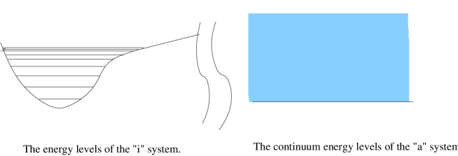
Figure 2: Discrete states coupled to a continuum

6.1 Relaxation of Density Matrix - Thermalization

We make the approximation namely that the $i$ system has only two states, $|0\rangle$ and $|1\rangle$. Furthermore we will assume that the continuum degrees are those of a continuum of harmonic oscillators. Harmonic oscillators are easy to analyze and also representative of the real situation where we expect $a$ degrees to be soft quanta. The frequencies of the harmonic oscillators are assumed to start at zero and form a continuum. In practice we just need the discrete spacing to be very small compared to the (inverse) time scales of interest. So if $\omega$ denotes the frequency of the oscillators, ${1\over\delta E_{a}}={1\over\delta\omega}>>T$. On the other hand $T$ should be large enough that the system has time to thermalize. In the previous section we saw that this time scale was set by $\gamma$. Thus $\gamma T>1$ and so $\delta\omega<<\gamma$. $\gamma$ in turn is fixed by the matrix elements $\langle 1,0|V|0,a\rangle$. Thus here also we require that the off diagonal terms generated by the interaction with the $a$ degrees of freedom must not be too small - this is expected whenever one has a resonance situation , i.e. $\hbar\omega=\Delta E$.

To do the calculation we will use the technique of influence functionals due to Feynman and Hibbs [37].

Following [37] we let $q$ be the coordinates of the $i$ system and $Q$ that of the $a$ system. If the system starts off at time $t=0$ in the state $\Psi(q_{i},Q_{i},0)$, then the density matrix at time $t=T$ is given by (The subscript $i$ stands for ‘initial’, and $f$ for ‘final’)

$$\rho(q_{f},q^{\prime}_{f},Q_{f},Q^{\prime}_{f};T)=\int...\int dq_{i}dq^{\prime}_{i}dQ_{i}dQ^{\prime}_{i}{\cal D}q(t){\cal D}q^{\prime}(t){\cal D}Q(t){\cal D}Q^{\prime}(t)$$

$$e^{i[S(q)-S(q^{\prime})]+i[S(Q)-S(Q^{\prime})]+i[S_{int}(Q,q)-S_{int}(Q^{\prime},q^{\prime})]}\Psi(q_{i},Q_{i},0)\Psi^{*}(q^{\prime}_{i},Q^{\prime}_{i},0)$$ (6.1.1)

with boundary conditions:

$$q(0)=q_{i},q(T)=q_{f},Q(0)=Q_{i},Q(T)=Q_{f}$$

$$q^{\prime}(0)=q^{\prime}_{i},q^{\prime}(T)=q^{\prime}_{f},Q^{\prime}(0)=Q^{\prime}_{i},Q^{\prime}(T)=Q^{\prime}_{f}$$ (6.1.2)

The action $S(q)$ for the $i$-system will not be specified. However we will assume, as stated before that there are only two discrete states $|0\rangle,|1\rangle$. We will further make the simplifying assumption that $\langle 0|q|0\rangle=\langle 1|q|1\rangle=0$ and that $\langle 0|q|1\rangle\neq 0$.

The $a$-system is a harmonic oscillator. Actually it is an infinite number of harmonic oscillators, so in fact there should be an infinite number of $Q$ variables. For transparency of presentation we first consider just one of them. As they are independent the generalization to arbitrary numbers or even a continuum is easy.

The wave function, $\Psi(q_{i},Q_{i},0)$, is assumed to factorize as

$$\Psi(q_{i},Q_{i},0)=\phi_{I}(q_{i})\chi_{a}(Q_{i})$$ (6.1.3)

Here

$$|\phi_{I}\rangle=\alpha|0\rangle+\beta|1\rangle$$ (6.1.4)

with $|\alpha|^{2}+|\beta|^{2}=1$. Let us first consider the case

$$\chi(Q)\approx e^{-{Q^{2}\over 2\omega}}$$ (6.1.5)

which is the ground state of a harmonic oscillator of frequency $\omega$. Furthermore we take $S_{int}(q,Q)\approx C\int dtq(t)Q(t)$.

We are interested in the density matrix traced over the $Q$ variables:

$$\int dQ_{f}\rho(q_{f},q^{\prime}_{f},Q_{f},Q_{f},T)\equiv\rho_{Q}(q_{f},q_{f}^{\prime},T)$$

If we imagine doing all the $Q,Q^{\prime}$ integrals we get an expression of the form

$$\rho_{Q}(q_{f},q^{\prime}_{f},T)=\int...\int dq_{i}dq^{\prime}_{i}{\cal D}q(t){\cal D}q^{\prime}(t)e^{i[S(q)-S(q^{\prime})]}\phi_{I}(q_{i})\phi^{*}_{I}(q^{\prime}_{i})F(q,q^{\prime}).$$ (6.1.6)

Here $F(q,q^{\prime})$ is the result of doing all the $Q$ integrals and incorporates the entire effect of the $Q$-system, called environment by Feynman and Hibbs, on the $q$-system. This is the influence functional. For the special case of quadratic $S(Q)$ and bilinear $S_{int}(q,Q)$ it has been shown in [37] that it has the form,

$$F(q,q^{\prime})=e^{-\int\int dtdt^{\prime}[q(t)-q^{\prime}(t)][\alpha(t,t^{\prime})q(t^{\prime})-\alpha^{*}(t,t^{\prime})q^{\prime}(t^{\prime})]}$$ (6.1.7)

For a harmonic oscillator of frequency $\omega$, in its ground state we have $\alpha(t,t^{\prime})=\alpha(t-t^{\prime})$ and also

$$\int d\tau e^{-i\nu\tau}\alpha(\tau)\equiv a(\nu)\approx{C\over\omega^{2}}\delta(\nu+\omega)$$ (6.1.8)

This is what Feynman and Hibbs call a cold-environment and for such a situations transitions pumping energy into the system are unlikely.

When we have a continuum of oscillators we simply have to integrate this expression (6.1.8) over $\omega$. We thus insert (6.1.7) into (6.1.6) and evaluate it perturbatively.

6.1.1 Zeroth Order

$$\rho_{00}=\int dq_{f}dq_{f}^{\prime}\phi_{0}^{*}(q_{f})\phi_{0}(q_{f}^{\prime})\rho_{Q}(q_{f},q^{\prime}_{f},T)$$

$$\rho_{10}=\int dq_{f}dq_{f}^{\prime}\phi_{1}^{*}(q_{f})\phi_{0}(q_{f}^{\prime})\rho_{Q}(q_{f},q^{\prime}_{f},T)$$ (6.1.9)

and so on. Thus

$$\langle 0|\rho|0\rangle=\langle 0|e^{-iHT}(\alpha|0\rangle+\beta|1\rangle)(\langle 0|\alpha^{*}+\langle 1|\beta^{*})e^{iHT}|0\rangle=|\alpha|^{2}$$ (6.1.10)

$$\langle 1|\rho|1\rangle=|\beta|^{2}$$ (6.1.11)

$$\langle 1|\rho|0\rangle=\langle 1|e^{-iHT}(\alpha|0\rangle+\beta|1\rangle)(\langle 0|\alpha^{*}+\langle 1|=\beta^{*})e^{iHT}|0\rangle=\alpha^{*}\beta e^{-i(E_{1}-E_{0})T}$$ (6.1.12)

$$\langle 0|\rho|1\rangle=\alpha\beta^{*}e^{+i(E_{1}-E_{0})T}$$ (6.1.13)

6.1.2 First Order

We now go to the next order. We bring down one power of $\alpha(t,t^{\prime})$.

We write it as the sum of four terms:

$$\delta\rho_{Qj0}(T)=-\int\int dq_{f}dq^{\prime}_{f}\phi^{*}_{j}(q_{f})\phi_{0}(q_{f}^{\prime})\int{\cal D}q(t){\cal=D}q^{\prime}(t)\int dq_{i}\int dq^{\prime}_{i}$$

$$e^{i[S(q)-S(q^{\prime})]}[a+b+c+d]\phi_{I}(q_{i})\phi_{I}^{*}(q^{\prime}_{i})$$ (6.1.14)

where the subscript $j$ on $\phi$ can be $0,1$ and

$$a = \int dt\int dt^{\prime}q(t)q(t^{\prime})\alpha(t,t^{\prime})$$

$$b = -\int dt\int dt^{\prime}q^{\prime}(t)q(t^{\prime})\alpha(t,t^{\prime})$$

$$c = -\int dt\int dt^{\prime}q(t)q^{\prime}(t^{\prime})\alpha^{*}(t,t^{\prime})$$

$$d = \int dt\int dt^{\prime}q^{\prime}(t)q(t^{\prime})\alpha^{*}(t,t^{\prime})$$ (6.1.15)

The calculations are done in the appendix. Here we will simply give the result.

We get for the first order correction to $\rho_{00}$ the following:

$$\delta\rho_{Q00}(T)=-T\{|\alpha|^{2}[2a_{R}(\Delta E)+2a_{R}(-\Delta E)]-2a_{R}(-\Delta E)\}|\langle 0|q|1\rangle|^{2}$$ (6.1.16)

where $\Delta E=E_{1}-E_{0}$, and

Let us first assume that $\Delta E>0$. Using (6.1.8), which says that $a_{R}(\Delta E)=0$, we find

$$\delta\rho_{Q00}(T)=-T[(|\alpha|^{2}-1)2a_{R}(-\Delta E)]|\langle 0|q|1\rangle|^{2}$$ (6.1.17)

This goes to zero when $|\alpha|\rightarrow 1$.

If $\Delta E<0$ we get

$$\delta\rho_{Q00}(T)=-T|\alpha|^{2}2a_{R}(\Delta E)|\langle 0|q|1\rangle|^{2}$$ (6.1.18)

When $E_{1}>E_{0}$ one expects the system to decay to its lower energy state $|0\rangle$ with the emission of a soft quanta. The decay stops when the probability of occupation of the lower energy state is one. Also as (6.1.17) shows $\delta\rho$ is increasing with time as it should be. Thus one expects $\beta(T)\approx\beta(0)e^{-\gamma T}$. So $|\alpha(T)|^{2}=1-|\beta(T)|^{2}\approx|\alpha(0)|^{2}+|\beta(0)|^{2}2\gamma T$. Thus $\delta\rho\approx|\beta(0)|^{2}2\gamma T$. This agrees with (6.1.17) for $\gamma=a_{R}(-\Delta E)|\langle 0|q|1\rangle|^{2}$.

Similarly when $E_{0}>E_{1}$, the probability of occupation of $E_{0}$ decreases with time as $|\alpha(T)|^{2}\approx|\alpha(0)|^{2}e^{-2\gamma T}$ and so $\delta\rho\approx-|\alpha(0)|^{2}2\gamma T$ as shown by (6.1.18).

Similarly we can look at the off diagonal terms

$$\delta\rho_{Q10}=-T\alpha^{*}\beta e^{-i(E_{1}-E_{0})T}|\langle 0|q|1\rangle|^{2}[a(-\Delta E)+a(\Delta E)^{*}]+$$

$$[\int_{0}^{T}d\tau e^{-i(E_{1}-E_{0})\tau}]\alpha\beta^{*}e^{-i(E_{1}-E_{0})T}(\langle 1|q|0\rangle)^{2}[a(0)+a(0)^{*}]$$ (6.1.19)

If $\Delta E\neq 0$, the integral over $\tau$ in the second term of (6.1.19) is vanishingly small relative to the first term. We are left with

$$\delta{\rho}_{Q10}=-T\alpha^{*}\beta e^{-i(E_{1}-E_{0})T}|\langle 0|q|1\rangle|^{2}[a(\Delta E)^{*}+a(-\Delta E)]$$ (6.1.20)

This is also as expected because the product $\alpha(T)\beta(T)$ decays as $e^{-\gamma T}$ (one of the terms decays and the other goes to 1).

While all this is as expected, this does not really demonstrate the De-coherence that we are after. In order to demonstrate decoherence we must show that the off diagonal terms decay even when the diagonal terms do not. In order to obtain a situation where the probabilities of occupation of the states $|0\rangle,|1\rangle$, are equal, one must have the external oscillators in excited states as well so that the system can absorb soft quanta. An easy route would be to let the two states be exactly degenerate so that energy conservation allows transitions in either direction. But in such a situation it is always possible to find orthonormal linear combinations of the two states in which the the operator $q$ is diagonal. It is then a simple exercise to show that in this basis the diagonal elements of the density matrix do not change at all. Even on physical grounds exact degeneracy is unreasonable to assume. What is more reasonable is to consider a situation in which $\Delta E\neq 0$ but ”small” compared to some relevant energy scale in the problem. Nevertheless, we need to calculate influence functionals for situations where the system can both absorb and give energy to the quantum environment. The influence functional calculated in Feynman and Hibbs for the case where all the environment oscillators are in the ground state will not suffice. While the generic case of the environment oscillators in arbitrary excited states is too difficult to handle, the influence function for the case where the environment states are coherent states or number states can be explicitly evaluated and this suffices for our purpose.

A partial form of this result is already available in Feynman and Hibbs (see eqn 8.141). They considered the amplitude $f(b,a)$ that a forced harmonic oscillator goes from state $f$ to state $g$ where

$$f(x)~{}=~{}({M\omega\over\pi\hbar})^{1\over 4}~{}e^{-({M\omega\over\pi\hbar})(x-a)^{2}}~{}~{}~{}~{}~{}~{}~{}~{}g(x)~{}=~{}({M\omega\over\pi\hbar})^{1\over 4}~{}e^{-({M\omega\over\pi\hbar})(x-b)^{2}}$$ (6.1.21)

Their explicit expression for $f(b,a)$ is

$$f(b,a)~{}=~{}A~{}e^{[-{M\omega\over 4\hbar}(a^{2}+b^{2}-2ab~{}e^{-i\omega T})+i({M\omega\over 2\hbar})^{1\over 2}(a\eta+b\eta^{*}e^{-i\omega T})]}$$ (6.1.22)

where

$$A~{}=~{}e^{-i\omega T/2}~{}e^{-{1\over 2M\omega\hbar}\int_{0}^{T}~{}\int_{0}^{t}~{}\gamma(t)\gamma(s)e^{-i\omega(t-s)}}$$ (6.1.23)

Of course, the states $f(x),g(x)$ are coherent states of the harmonic oscillator but with real parameters. It suffices, for our purposes, to generalise this result to the case where $f(x)$ is a coherent state with complex parameter $\xi$ while leaving $b$ still real. The corresponding results are

$$f(x)~{}=~{}({M\omega\over\pi\hbar})^{1\over 4}~{}e^{{\xi^{2}\over 2}-{|\xi|^{2}\over 2}}~{}e^{-({M\omega\over\pi\hbar})(x-\sqrt{{2\hbar\over M\omega}}~{}\xi)^{2}}~{}~{}~{}~{}~{}~{}~{}~{}$$ (6.1.24)

where we have followed the Pancharatnam convention for phases.

$$f(b,\xi)~{}=~{}{\cal A}~{}e^{[-{M\omega\over 4\hbar}({2\hbar\over M\omega}\xi^{2}+b^{2}-2\sqrt{{2\hbar\over M\omega}}\xi b~{}e^{-i\omega T})+i({M\omega\over 2\hbar})^{1\over 2}(\sqrt{{2\hbar\over M\omega}}\xi\eta+b\eta^{*}e^{-i\omega T})]}$$ (6.1.25)

where

$${\cal A}~{}=~{}e^{{\xi^{2}\over 2}-{|\xi|^{2}\over 2}}~{}e^{-i\omega T/2}~{}e^{-{1\over 2M\omega\hbar}\int_{0}^{T}~{}\int_{0}^{t}~{}\gamma(t)\gamma(s)e^{-i\omega(t-s)}}$$ (6.1.26)

Now it is easily seen that $G_{0\xi},G_{m\xi}$ where $G_{fi}$ is the amplitude that the oscillator initially in state $i$ is found in state $f$ at time T, are given by

$$G_{0\xi}=~{}e^{-{|\xi|^{2}\over 2}+i\xi\eta}~{}e^{-{1\over 2M\omega\hbar}\int_{0}^{T}~{}\int_{0}^{t}~{}\gamma(t)\gamma(s)e^{-i\omega(t-s)}}$$ (6.1.27)

and

$$G_{m\xi}=~{}{1\over{\sqrt{m!}}}~{}G_{0\xi}~{}(\xi+i\eta^{*})^{m}$$ (6.1.28)

Finally the influence functional is given by

$$F[q,q^{\prime}]~{}=~{}\sum_{m}~{}G_{m\xi}{G^{\prime}_{m\xi}}^{*}$$ (6.1.29)

The final result can be expressed as

$$F_{\xi}[q,q^{\prime}]~{}~{}e^{i\xi(\eta-\eta^{\prime})+i\xi^{*}(\eta^{*}-{\eta^{\prime}}^{*})}~{}F_{0}[q,q^{\prime}]$$ (6.1.30)

where $F_{0}$ is the influence functional for the case where the environment oscillators are in the ground state.

Thus the environmental coherent states produce an additional influence functional whose exponent is a linear functional of $q$. However, to the degree of accuracy needed for our perturbative calculations we can translate this into an effective quadratic functional by expanding the additional term to second order i.e

$$-{1\over 4M^{2}\omega}[\xi^{2}~{}(\eta-\eta^{\prime})^{2}+{\xi^{*}}^{2}~{}(\eta^{*}-{\eta^{\prime}}^{8})^{2}+2|\xi|^{2}~{}|(\eta-\eta^{\prime})|^{2}]$$

It is sufficient to look at terms of the type

$$\int_{0}^{T}~{}dt\int_{0}^{t}~{}ds\Delta a(t,s)q(t)q(s)$$

to determine the one complex function $\Delta a(t,s)$ that determines the additional effective influence functional. After some algebra it follows that

$$\Delta a(t,s)~{}=~{}{C^{2}\over 4M^{2}\omega}~{}[2\xi^{2}e^{-i\omega(t+s)}+2{\xi^{*}}^{2}e^{i\omega(t+s)}+2|\xi|^{2}(e^{i\omega(t-s)}+e^{-i\omega(t-s)}]$$ (6.1.31)

Unlike the case of the environment oscillators in the ground state the complex function is not a function of $t-s$ alone but it turns out that the parts of $a(t,s)$ that are functions of $t+s$ do not contribute to the transition rates as the integrations over $s,t$ produce mutually exclusive delta functions and one is effectively left with

$$\Delta a_{eff}(t,s)~{}=~{}{C^{2}\over 4M^{2}\omega}~{}2|\xi|^{2}[(e^{i\omega(t-s)}+e^{-i\omega(t-s)}]$$ (6.1.32)

Thus when the environmental oscillators are in coherent states we have a mixture of a cold-environment whose strength is independent of the coherent state parameter $\xi$ and a classical noise environment with $a_{R}(\nu)=a_{R}(-\nu)$. Further $a_{R}(\nu)$ is directly proportional to the level of excitation of the coherent states. It should be emphasised that any environment can be represented as a mixture of a cold environment and a classical noise environment. But what is special about the coherent state case is that the cold component is independent of the level of excitation of the coherent states. This will be crucial for us later on.

In the number state case, there are no $t+s$ terms to begin with (as shown on the Appendix) and one obtains (B.28) directly - this is (6.1.32) with $|\xi|^{2}$ replaced by $m$, the excitation number of the oscillator.

If we use (B.28) (or (6.1.32)), with large $m$ or $|\xi|^{2}$, we can neglect the cold term in the influence functional. In this case $a_{R}(\Delta E)=a_{R}(-\Delta E)$, and both are non-zero. Then we see from (6.1.20) that

$$\delta\rho_{Q00}=-T(2|\alpha|^{2}-1)|\langle 0|q|1\rangle|^{2}2a_{R}(\Delta E)$$

$$\delta\rho_{Q01}=-T\underbrace{\alpha^{*}\beta e^{-i\Delta ET}}_{\rho_{Q01}}|\langle 0|q|1\rangle|^{2}2a_{R}(\Delta E)$$

$$\approx~{}\rho_{Q01}(e^{-\gamma T}-1)$$ (6.1.33)

Thus in this approximation even when $|\alpha|^{2}={1\over 2}$, $\delta\rho_{Q01}\neq 0$. Equation (6.1.33), if our extrapolation from the linear term to the full exponential is correct, demonstrates decoherence. To actually prove decoherence one would have get a more complete solution. Presumably this can be done numerically in some cases.

Thus we have evidence for decoherence in an explicit calculation in this simplified model. The crucial point here is the appearance of the imaginary term due to “absorption of a soft quanta by the environment”. We have put the quotation marks because this is really just a convenient trick. We have made a division into two sets of variables $i$ and $a$ with the requirement that $a$ should have a continuous spectrum We called these “soft quanta”. Then we showed that the same mathematical manipulations that give rise to an imaginary part to the energy of a discrete state can be used here to show that the off-diagonal terms of the density matrix decay.

We should also check that the conditions set forth at the end of the last section are indeed satisfied. $\delta_{a}$ is zero for this calculation. Due to resonance, the off-diagonal terms are large. Thus both conditions are satisfied. While we have not proved even in a non-rigourous way, the existence of the phenomenon of self thermalization, the calculations done here do make plausible the physical ideas of section 2 and also buttress the intuitive random phase arguments about the off diagonal terms of the density matrix decaying in time, that were made in section 3.

7 Conclusions

In this paper we have attempted to provide a physical picture of the process of self thermalization, by which a pure state can appear thermal if studied with coarse resolution. This phenomenon underlies the validity of the microcanonical ensemble in quantum statistical mechanics. It also has applications in the black hole information paradox.

We have presented an intuitive physical picture along with a mathematical formulation of the process. The principal new ingredient was the introduction of dynamical “soft quanta” that are not included in the microstate descriptions. They are coarse grained away and in the process, remove correlations between the (coarse grained) microstates. Thus they not only provide the quantum analogue of the Gibbsian coarse graining of microstates (Section 4), they also thermalize the system by resonant absorpton and emission (Section 5,6). Mathematically this is identical to the appaearance of an imaginary part in the energy of an excited state when it couples to a continuum. This also provides a way to calculate the thermalization rate. A first order perturbation calculation (Section 6) supports this picture.

It would be interesting to apply this picture to some interesting systems in a quantitative way. This would be a test of the correctness of these ideas.

Acknowledgements
We would like to thank Balram Rai and R. Shankar for discussions.

Appendix A Appendix: Density Matrix Calculation

In this appendix we derive (6.1.16) and (6.1.19) starting from (6.1.14).

We will first work out in detail the contribution of the perturbation labelled ‘$a$’.

The $q$ and $q^{\prime}$ integrals can be done separately. Let us denote by $A_{j}$ the $q$ integral and by $A^{\prime}$ ($A^{\prime\prime}$ does not depend on $j$) the $q^{\prime}$ integral. Thus

$$A_{j}=\int dq_{f}\phi^{*}_{j}(q_{f}){\cal D}qe^{iS(q)}\int dq_{i}q(t)q(t^{\prime})\phi_{I}(q_{i})$$

$$A^{\prime}=\int dq^{\prime}_{f}\phi_{0}(q^{\prime}_{f}){\cal D}q^{\prime}(t)e^{-iS(q^{\prime})}dq^{\prime}_{i}\phi_{I}^{*}(q^{\prime}_{i})$$

$$\delta\rho_{Qj0}(T)=\int_{0}^{T}dt\int_{0}^{T}dt^{\prime}\alpha(t,t^{\prime})A_{j}A^{\prime}$$ (A.1)

$\bf A_{j}:$

$$A_{j}=\int dq_{f}\int dq_{i}\phi^{*}_{j}(q_{f})\int{\cal D}qe^{iS(q)}q(t)q(t^{\prime})\phi_{I}(q_{i})$$

$$=\sum_{m=0,1}\langle j|e^{-iH(T-t)}q|m\rangle e^{-iH(t-t^{\prime})}\langle m|qe^{-iHt^{\prime}}(\alpha|0\rangle+\beta|1\rangle)$$

If $j=0$ we get

$$A_{0}=\langle 0|e^{-i(E_{0}(T-t)}q|1\rangle e^{-iE_{1}(t-t^{\prime})}\langle 1|qe^{-iE_{0}t^{\prime}}\alpha|0\rangle$$

$$=e^{-iE_{0}T}e^{-i(E_{1}-E_{0})(t-t^{\prime})}\langle 0|q|1\rangle\langle 1|q|0\rangle\alpha$$ (A.2)

If $j=1$ we get

$$A_{1}=\langle 1|e^{-iE_{1}(T-t)}q|0\rangle e^{-iE_{0}(t-t^{\prime})}\langle 0|qe^{-iE_{1}t^{\prime}}\beta|1\rangle$$

$$=e^{-iE_{1}T}e^{-i(E_{0}-E_{1})(t-t^{\prime})}\langle 1|q|0\rangle\langle 0|q|1\rangle\beta$$ (A.3)

$\bf A^{\prime}:$

$$A^{\prime}=[\int dq^{\prime}_{f}{\cal D}q^{\prime}(t)dq^{\prime}_{i}\phi_{I}(q^{\prime}_{i})e^{iS(q^{\prime})}\phi_{i}^{*}(q^{\prime}_{f})]^{*}$$

$$=[\langle 0|e^{-iHT}(\alpha|0\rangle+\beta|1\rangle)]^{*}=\alpha^{*}e^{iE_{0}T}$$ (A.4)

Combining all the above we get the contribution due to the perturbation $a$. :

$$\delta\rho_{Q00}(T)=|\alpha|^{2}\int_{0}^{T}dt\int_{0}^{T}dt^{\prime}e^{-i(E_{1}-E_{0})(t-t^{\prime})}\alpha(t-t^{\prime})|\langle 1|q|0\rangle|^{2}$$

$$=T|\alpha|^{2}|\langle 1|q|0\rangle|^{2}a(E_{1}-E_{0})$$ (A.5)

and

$$\delta\rho_{Q10}(T)=\alpha^{*}\beta e^{-i(E_{1}-E_{0})T}\int_{0}^{T}dt\int_{0}^{T}dt^{\prime}e^{-i(E_{0}-E_{1})(t-t^{\prime})}\alpha(t-t^{\prime})|\langle 1|q|0\rangle|^{2}$$

$$=T\alpha^{*}\beta|\langle 1|q|0\rangle|^{2}a(E_{0}-E_{1})e^{-i(E_{1}-E_{0})T}$$ (A.6)

We can similarly calculate the contribution from the other ones.

$\bf B_{j}:$

$$B_{0}=\langle 0|e^{-iH(T-t^{\prime})}q|m\rangle e^{-iE_{m}t^{\prime}}\langle m|(\alpha|0\rangle+\beta|1\rangle)$$

$$=\beta e^{-iE_{0}T}e^{-i(E_{1}-E_{0})t^{\prime}}\langle 0|q|1\rangle$$ (A.7)

$$B_{1}=\langle 1|e^{-iH(T-t^{\prime})}q|m\rangle e^{-iE_{m}t^{\prime}}\langle m|(\alpha|0\rangle+\beta|1\rangle)$$

$$=\alpha e^{-iE_{1}T}e^{-i(E_{0}-E_{1})t^{\prime}}\langle 1|q|0\rangle$$ (A.8)

$\bf B^{\prime}:$

$$B^{\prime}=[\int dq^{\prime}_{f}\phi_{i}^{*}(q^{\prime}_{f}){\cal D}q^{\prime}(t)dq^{\prime}_{i}e^{iS(q^{\prime})}\phi_{I}(q^{\prime}_{i})]^{*}$$

$$=[\langle 0|e^{-iH(T-t)}q^{\prime}|m\rangle e^{-iE_{m}t}\langle m|(\alpha|0\rangle+\beta|1\rangle)]^{*}$$

$$=\beta^{*}e^{+iE_{0}T}\langle 1|q|0\rangle e^{-i(E_{0}-E_{1})t}$$ (A.9)

Combining the above

$$\delta\rho_{Q00}=T|\beta|^{2}|\langle 0|q|1\rangle|^{2}a(E_{0}-E_{1})$$ (A.10)

and

$$\delta\rho_{Q10}=[\int_{0}^{T}d\tau e^{-i(E_{0}-E_{1})\tau}]\alpha\beta^{*}e^{-i(E_{1}-E_{0})T}(\langle 1|q|0\rangle)^{2}a(0)$$ (A.11)

(Note that the factor inside the square brackets replaces the factor $T$ that appeared in previous terms.)

$\bf C_{j}:$

$$C_{0}=\langle 0|e^{-iH(T-t)}q|m\rangle e^{-iE_{m}t}\langle m|(\alpha|0\rangle+\beta|1\rangle)$$

$$=\beta e^{-iE_{0}T}e^{-i(E_{1}-E_{0})t}\langle 0|q|1\rangle$$ (A.12)

$$C_{1}=\langle 1|e^{-iH(T-t)}q|m\rangle e^{-iE_{m}t}\langle m|(\alpha|0\rangle+\beta|1\rangle)$$

$$=\alpha e^{-iE_{1}T}e^{-i(E_{0}-E_{1})t}\langle 1|q|0\rangle$$ (A.13)

$\bf C^{\prime}:$

$$C^{\prime}=[\int dq^{\prime}_{f}\phi_{i}^{*}(q^{\prime}_{f}){\cal D}q^{\prime}(t^{\prime})dq^{\prime}_{i}e^{iS(q^{\prime})}\phi_{I}(q^{\prime}_{i})]^{*}$$

$$=[\langle 0|e^{-iH(T-t^{\prime})}q^{\prime}|m\rangle e^{-iE_{m}t^{\prime}}\langle m|(\alpha|0\rangle+\beta|1\rangle)]^{*}$$

$$=\beta^{*}e^{+iE_{0}T}e^{-i(E_{0}-E_{1})t^{\prime}}\langle 1|q|0\rangle$$ (A.14)

Combining:

$$\delta\rho_{Q00}=T|\beta|^{2}|\langle 0|q|1\rangle|^{2}[a(E_{0}-E_{1})]^{*}$$ (A.15)

$$\delta\rho_{Q10}=[\int_{0}^{T}d\tau e^{-i(E_{0}-E_{1})\tau}]\alpha\beta^{*}e^{-i(E_{1}-E_{0})T}(\langle 1|q|0\rangle)^{2}a^{*}(0)$$ (A.16)

$\bf D_{j}:$

$$D_{0}=\langle 0|e^{-iHT}(\alpha|0\rangle+\beta|1\rangle)=\alpha e^{-iE_{0}T}$$ (A.17)

$$D_{1}=\langle 1|e^{-iHT}(\alpha|0\rangle+\beta|1\rangle)=\beta e^{-iE_{1}T}$$ (A.18)

$\bf D^{\prime}:$

$$D^{\prime}=[\int dq^{\prime}_{f}\phi_{i}^{*}(q^{\prime}_{f}){\cal D}q^{\prime}(t)q^{\prime}(t^{\prime})dq^{\prime}_{i}e^{iS(q^{\prime})}\phi_{I}(q^{\prime}_{i})]^{*}$$

$$=[\langle 0|e^{-iH(T-t)}q^{\prime}|m\rangle e^{-iE_{m}(t-t^{\prime})}\langle m|qe^{-iHt^{\prime}}(\alpha|0\rangle+\beta|1\rangle)]^{*}$$

$$=\alpha^{*}e^{iE_{0}T}e^{-i(E_{0}-E_{1})(t-t^{\prime})}|\langle 0|q|1\rangle|^{2}$$ (A.19)

Combining:

$$\delta\rho_{Q00}=T|\alpha|^{2}|\langle 0|q|1\rangle|^{2}[a(E_{1}-E_{0})]^{*}$$ (A.20)

$$\delta\rho_{Q10}=T\alpha^{*}\beta|\langle 1|q|0\rangle|^{2}[a(E_{1}-E_{0})]^{*}e^{-i(E_{1}-E_{0})T}$$ (A.21)

If we add up all the contributions $a+b+c+d$ we get the expressions (6.1.16) and (6.1.19).

Appendix B Appendix: Influence Functional Calculation

In this Appendix we will derive the influence functional for the cases when the ”external” oscillators are either in coherent states or in number eigenstates.

We start with the kernel $K(Q_{f},Q_{i},Cq)$ for a forced harmonic oscillator forced with $f(t)=Cq(t)$ given by

$$K=\underbrace{{\sqrt{M\omega\over 2\pi i\hbar sin~{}\omega T}}}_{N}e^{{i\over\hbar}S_{cl}(Q_{f},Q_{i},Cq)}$$ (B.1)

As shown in [37] $S_{cl}$ is given by,

$$S_{cl} = {M\omega\over 2sin~{}\omega T}[cos~{}\omega T(Q_{f}^{2}+Q_{i}^{2})-2Q_{f}Q_{i}$$ (B.2)

$$+ {2Q_{f}C\over M\omega}\int_{0}^{T}q(t)sin~{}\omega t~{}dt+{2Q_{i}C\over M\omega}\int_{0}^{T}q(t)sin~{}\omega(T-t)~{}dt$$

$$- {C^{2}\over M^{2}\omega^{2}}\int_{0}^{T}\int_{0}^{t}q(t)q(s)sin~{}\omega(T-t)sin~{}\omega s~{}ds~{}dt]$$

We need to calculate the following quantity:

$$\int dQ_{f}dQ_{i}dQ^{\prime}_{i}|N|^{2}e^{{i\over\hbar}[S_{cl}(Q_{f},Q_{i},Cq)-S_{cl}(Q_{f},Q^{\prime}_{i},Cq^{\prime})}\psi(Q_{i})\psi^{*}(Q_{i}^{\prime})$$ (B.3)

The $Q$ oscillator starts off at time $t=0$ in a state $\psi$. The density matrix at time $T$ is then traced over the coordinates of the $Q$ oscillator. For $\psi(Q_{i})$ we use the coherent states. Thus we use

$$f(x)~{}=~{}({M\omega\over 2\hbar})^{1\over 4}~{}e^{{\xi^{2}\over 2}-{|\xi|^{2}\over 2}}~{}e^{-({M\omega\over 2\hbar})(x-\sqrt{{2\hbar\over M\omega}}~{}\xi)^{2}}~{}~{}~{}~{}~{}~{}~{}~{}$$ (B.4)

where we have followed the Pancharatnam convention for phases. It should be noted that eqn (B.3) straightaway gives the influence functional. The method followed in [37] is needlessly circuitous. After obtaining the nonperturbative expression for the coherent case influence functional which will be shown to have a part linear in $q(t),q^{\prime}(t)$, we will introduce an effective influence functional quadratic in $q(t),q^{\prime}(t)$ that is obtained perturbatively. We will obtain expressions for this effective influence functional both for the coherent states as well as for the number states.

The $Q$-dependent terms in the integrand in (B.3) can be written as

$$e^{-{1\over 2}[AQ_{f}^{2}+BQ_{i}^{2}+C{Q^{\prime}}_{i}^{2}+2DQ_{f}Q_{i}+2EQ_{f}Q^{\prime}_{i}]+FQ_{f}+GQ_{i}+HQ^{\prime}_{i}}$$ (B.5)

with

$$A=0,~{}~{}B=-{M\omega\over\hbar\sin{\omega T}}ie^{i\omega T},~{}~{}C=B^{*},$$ (B.6)

$$D={iM\omega\over\hbar\sin{\omega T}}~{}~{},~{}~{}E=D^{*}$$ (B.7)

$$F={iC\over\hbar\sin{\omega T}}\int_{0}^{T}(q-q^{\prime})\sin{\omega t}~{}dt,$$ (B.8)

$$G={iC\over\hbar\sin{\omega T}}\int_{0}^{T}qsin~{}\omega(T-t)~{}dt~{}+~{}\sqrt{{2M\omega\over\hbar}}\xi$$ (B.9)

$$H={-iC\over\hbar\sin{\omega T}}\int_{0}^{T}q^{\prime}sin~{}\omega(T-t)~{}dt~{}+~{}\sqrt{{2M\omega\over\hbar}}\xi^{*}$$ (B.10)

The result of doing the Gaussian integral is

$$\sqrt{{(2\pi)^{3}\over 2}({\hbar\over M\omega})^{3}sin^{2}~{}\omega T}~{}~{}e^{{\hbar\over 4M\omega}[F^{2}+(G+H)^{2}+e^{-i\omega T}2FG+e^{i\omega T}2FH]}$$ (B.11)

The overall normalisation factor is

$${\cal N} = |N|^{2}~{}\sqrt{{(2\pi)^{3}\over 2}({\hbar\over M\omega})^{3}sin^{2}~{}\omega T}~{}~{}({M\omega\over\pi\hbar})^{1/2}~{}e^{\xi^{2}/2+{\xi^{*}}^{2}/2-|\xi|^{2}}$$ (B.12)

$$= e^{\xi^{2}/2+{\xi^{*}}^{2}/2-|\xi|^{2}}$$

Thus the final result is

$${\cal N}exp\{{\hbar\over 4M\omega}[F^{2}+(G+H)^{2}+e^{-i\omega T}2FG+e^{i\omega T}2FH]$$ (B.13)

$$- {i\over\hbar\sin{\omega T}}{C^{2}\over M\omega}\int_{0}^{T}\int_{0}^{t}q(t)q(s)sin~{}\omega(T-t)sin~{}\omega s~{}ds~{}dt$$

$$+ {i\over\hbar\sin{\omega T}}{C^{2}\over M\omega}\int_{0}^{T}\int_{0}^{t}q^{\prime}(t)q^{\prime}(s)sin~{}\omega(T-t)sin~{}\omega s~{}ds~{}dt\}$$

As shown in [37] the influence functional for this class of problems has the general form

$$F(q,q^{\prime})=\int_{0}^{T}\int_{0}^{t}[q(t)-q^{\prime}(t)][a(t,s)q(s)-a^{*}(t,s)q^{\prime}(s)]~{}dt~{}ds$$ (B.14)

Thus we can extract $a(t,s)$ from the $q(t)q(s)$ terms. Calculationally it is easier to look at the $q(t)q^{\prime}(s)$ terms to get $a(t,s)$ as the terms in $S_{cl}$ that are quadratic in $q(t)$ do not contribute. We find for the $\alpha$ independent part of the $q(t)q(s)$ term the following sum of four terms(an overall factor of ${C^{2}\over M\omega}$ has been suppressed for the moment):

$$-{1\over 2sin^{2}~{}\omega T}\int_{0}^{T}\int_{0}^{t}q(t)q(s)sin~{}\omega tsin~{}\omega s$$

$$-{1\over 2sin^{2}~{}\omega T}\int_{0}^{T}\int_{0}^{t}q(t)q(s)sin~{}\omega(T-t)sin~{}\omega(T-s)$$

$$-{e^{\i\omega T}\over 2sin^{2}~{}\omega T}\int_{0}^{T}\int_{0}^{t}q(t)q(s)[sin~{}\omega tsin~{}\omega(T-s)+sin~{}\omega ssin~{}\omega(T-t)]$$

$$-{i\over sin~{}\omega T}\int_{0}^{T}\int_{0}^{t}q(t)q(s)sin~{}\omega(T-t)sin~{}\omega s$$ (B.15)

These can be rewritten as functions of $t-s$ and $t+s$. The $t-s$ terms are(after restoring all factors)

$$- {C^{2}\over M\omega}{1\over 4sin^{2}~{}\omega T}[2cos~{}\omega(t-s)-{e^{-i\omega T}}cos~{}\omega(T-s+t)$$ (B.16)

$$- {e^{-i\omega T}}cos~{}\omega(T-t+s)-2i\sin{\omega T}cos~{}\omega(T-t+s)]$$

They add up to

$$-{C^{2}\over M\omega}[{cos~{}\omega(t-s)\over 2}+i{sin~{}\omega(t-s)\over 2}]=-{C^{2}\over 2M\omega}e^{i\omega(t-s)}$$ (B.17)

This is the influence functional when the $Q$-oscillator is in its ground state [37]. We also have to check that the $t+s$ terms are zero The $t+s$ terms are

$${1\over 4sin^{2}~{}\omega T}cos~{}\omega(t+s)+{1\over 4sin^{2}~{}\omega T}cos~{}\omega(2T-t-s)$$ (B.18)

$${ie^{-i\omega T}\over 2sin^{2}~{}\omega T}cos~{}\omega(T-s-t)-{i\over 2sin\omega T}cos\omega(T-t-s)$$

They can be seen to add up to zero.

Now we turn to the $\xi$-dependent terms.First let us look at the terms quadratic in $\xi$:

$${\hbar\over 4M\omega}[({2M\omega\over\hbar})(\xi+\xi^{*})^{2}]={1\over 2}(\xi+\xi^{*})^{2}$$

the exponential of which exactly cancels the factor ${\cal N}$.

(B.19)

Now we look at the terms linear in $\xi$:

$${\hbar\over 4M\omega}[2F\sqrt{{2M\omega\over\hbar}}(\xi e^{-i\omega T}+\xi^{*}e^{i\omega T})+2\sqrt{{2M\omega\over\hbar}}(\xi+\xi^{*}){iC\over\hbar\sin{\omega T}}\int_{0}^{T}\sin{\omega(T-t)}(q-q^{\prime})]$$

On using the expression for $F$ and some rearrangement it is easy to see that this equals

$${iC\over\hbar}\sqrt{{\hbar\over 2M\omega}}\int_{0}^{T}dt~{}(q(t)-q^{\prime}(t))(\xi e^{-i\omega T}+\xi^{*}e^{i\omega T})$$ (B.20)

which can be reexpressed as

$$iC\xi(\eta-\eta^{\prime})+iC\xi^{*}(\eta^{*}-{\eta^{\prime}}^{*})$$ (B.21)

where

$$\eta=\sqrt{{1\over 2M\omega\hbar}}\int_{0}^{T}dt~{}q(t)e^{-i\omega t}$$ (B.22)

We can thus express the influence functional for the case when the $Q$-oscillator is in the coherent state as

$$F_{\xi}(q,q^{\prime})=F_{0}(q,q^{\prime})~{}e^{iC\xi(\eta-\eta^{\prime})+iC\xi^{*}(\eta^{*}-{\eta^{\prime}}^{*})}$$ (B.23)

with $\eta$ given by eqn (B.22). Within perturbation theory we can expand the exponential of the linear functional in $q,q^{\prime}$.It turns out that the linear term does not contribute and the quadratic terms are:

$$-{1\over 4M^{2}\omega}[\xi^{2}~{}(\eta-\eta^{\prime})^{2}+{\xi^{*}}^{2}~{}(\eta^{*}-{\eta^{\prime}}^{8})^{2}+2|\xi|^{2}~{}|(\eta-\eta^{\prime})|^{2}]$$

It is sufficient to look at terms of the type

$$\int_{0}^{T}~{}dt\int_{0}^{t}~{}ds{\Delta a(t,s)}_{coh}q(t)q(s)$$

to determine the one complex function ${\Delta a(t,s)}_{coh}$ that determines the additional effective influence functional. After some algebra it follows that

$${\Delta a(t,s)}_{coh}~{}=~{}{C^{2}\over 4M^{2}\omega}~{}[2\xi^{2}e^{-i\omega(t+s)}+2{\xi^{*}}^{2}e^{i\omega(t+s)}+2|\xi|^{2}(e^{i\omega(t-s)}+e^{-i\omega(t-s)}]$$ (B.24)

Now we turn to the evaluation of the effective influence functional when the $Q$-oscillators are in the $m$-th number state $|m\rangle$. For this we recall the expansion of the coherent state $|\xi\rangle$ in terms of the number states:

$$|\xi\rangle=e^{-|\xi|^{2}/2}\sum_{n}~{}{\xi^{n}\over\sqrt{n!}}|n\rangle$$ (B.25)

Thus

$$F_{\xi}(q,q^{\prime})=e^{-|\xi|^{2}}\sum_{n,m}{\xi^{n}\over\sqrt{n!}}{{\xi^{*}}^{m}\over\sqrt{m!}}~{}F_{m,n}(q,q^{\prime})$$ (B.26)

Therefore to get the influence functional(in the perturbative sense described above) for the case in which the $Q$-oscillators are in the state $|m\rangle$ one has to expand $e^{|\xi|^{2}}~{}F_{\xi}$ in powers of $|\xi|^{2}$(and quadratic in $q(t)$ and pick the coefficient of $|\xi|^{2m}$.The $m$-th term of the expansion is

$${|\xi|^{2m}\over m!}~{}a_{0}(t,s)+{|\xi|^{2(m-1)}\over(m-1)!}~{}C^{2}|\eta|^{2}$$ (B.27)

It is elementary to show that

$$a_{m}(t,s)=a_{0}(t,s)+m{C^{2}\over M\omega}(e^{i\omega(t-s)}+e^{-i\omega(t-s)})$$ (B.28)

References

- [1] S. Kalyana Rama and B. Sathiapalan, On the Role of Chaos in the AdS/CFT Connection Int. J. Mod. Phys. A14 (1999) 2635, hep-th/9905219.
- [2] J. Maldacena, Adv. Theor. Math. Phys. 2(1998), hep-th/9711200.
- [3] E. Witten, Adv. Theor. Math. Phys. 2(1998), hep-th/9802150.
- [4] L.E. Reichl, ”A Modern Course in Statistical Physics”, University of Texas Press, Austin, p.241.
- [5] Ya. G. Sinai in the The Boltzmann Equation,ed. E.G.D. Cohen and W. Thirring(Springer- Verlag, Vienna, 1973).
- [6] Paul and Tatiana Ehrenfest,The Conceptual Foundations of the Statistical Approach in Mechanics,Cornell University Press,Ithaca,New York,1959.
- [7] J.W. Gibbs,”Elementary Principles in Statistical Mechanics”, Dover Edition, 1960.
- [8] V.I. Arnold, ”Mathematical Foundations of Classical Mechanics”, Springer-Verlag,1980, p.71.
- [9] S. Chandrasekhar, Rev. Mod. Phys. 15 1(1943).
- [10] J.v. Neumann, Zeitschrift fur Physik, 57, 30, 1929.
- [11] Sommerfeld Festschrift(Leipzig 1928) p.30; W. Pauli and M. Fierz, Zeits. Phys.106 5721937.
- [12] N.G. Van Kampen Fundamental Problems in Statistical Mechanics of Irreversible Processes in Fundamental Problems in Statistical Mechanics, ed.E.G.D. Cohen,North-Holland Publishing Company,1962.
- [13] T. S. Biro, S. G. Matinyan and B. Mueller, “Chaos and Gauge Field Theory”, (1994),World Scientific, Singapore ; T. S. Biro, C. Gong and B. Mueller, Phys. Rev. D52 (1995) 1260, hep-ph/940932.
- [14] B. Mueller and A. Trayanov, Phys. Rev. Lett. 68 (1992) 3387 ; T.S.Biro, M. Feurstein, H. Markum, hep-lat/9711002.
- [15] V.V.Flambaum and F.M.Izrailev, Time dependence of occupation numbers and thermalization time in closed chaotic many-body systems, quant-ph/0108109.
- [16] V.V.Flambaum and F.M.Izrailev, Entropy production and wave packet dynamics in the Fock space of closed chaotic many-body systems, quant-ph/0103129.
- [17] F.M.Izrailev, Quantum Chaos and Thermalization for Interacting Particles, lectures given in the CXLIII Course ”New Directions in Quantum Chaos” on the International School of Physics ”Enrico Fermi”; Varenna, Italy, July 1999; to be published in Proceedings; cond-mat/9911297.
- [18] Doron Cohen, Felix M. Izrailev, and Tsampikos Kottos, Wavepacket dynamics in energy space, RMT and quantum-classical correspondence, Phys. Rev. Lett. 84 (2000) 2052; chao-dyn/9909015.
- [19] V. V. Flambaum, A. A. Gribakina, G. F. Gribakin, and I. V. Ponomarev, Interaction-Driven Equilibrium and Statistical Laws in Small Systems. The Cerium Atom, Phys. Rev. E 57 (1998) 4933; cond-mat/9711213.
- [20] F.Borgonovi, I.Guarneri, F.M.Izrailev, and G.Casati, Chaos and Thermalization in a Dynamical Model of Two Interacting Particles, chao-dyn/9711005.
- [21] V.V. Flambaum and F.M. Izrailev, Distribution of occupation numbers in finite Fermi-systems and role of interaction in chaos and thermalization, Phys. Rev. E 55 (1997) R13; cond-mat/9610178.
- [22] Jochen Gemmer, Alexander Otte, and Guenter Mahler, Quantum Approach to a Derivation of the Second Law of Thermodynamics, quant-ph/0101140.
- [23] D. L. Shepelyansky, Quantum Chaos & Quantum Computers, Physica Scripta T90 (2001) 112; quant-ph/0006073.
- [24] B. Georgeot and D. L. Shepelyansky, Emergence of Quantum Chaos in Quantum Computer Core and How to Manage It, quant-ph/0005015.
- [25] Ph. Jacquod and D. L. Shepelyansky, Emergence of quantum chaos in finite interacting Fermi systems, cond-mat/9706040.
- [26] G. A. Luna-Acosta and J. A. Mendez-Bermudez, F. M. Izrailev, Periodic Chaotic Billiards: Quantum-Classical Correspondence in Energy Space, Phys. Rev. E 64 (2001) 036206; cond-mat/0105108.
- [27] G. A. Luna-Acosta, J. A. Mendez-Bermudez, and F. M. Izrailev, Quantum-classical correspondence for local density of states and eigenfunctions of a chaotic periodic billiard, Phys. Lett. A 274 (2000) 192-199; nlin.CD/0002044.
- [28] B. Mehlig and M. Santer, Universal eigenvector statistics in a quantum scattering ensemble, cond-mat/0012025.
- [29] Don N. Page, Average Entropy of a Subsystem, Phys.Rev.Lett. 71 (1993) 1291; gr-qc/9305007.
- [30] Siddhartha Sen, Average Entropy of a Subsystem, Phys.Rev.Lett. 77 (1996) 1; hep-th/9601132.
- [31] Mark Srednicki, The approach to thermal equilibrium in quantized chaotic systems, J. Phys. A 32 (1999) 1163, cond-mat/9809360; Thermal Fluctuations in Quantized Chaotic Systems, J.Phys. A 29 (1996) L75, chao-dyn/9511001; Does Quantum Chaos Explain Quantum Statistical Mechanics?, cond-mat/9410046; Quantum Chaos and Statistical Mechanics, talk given at the Conference on Fundamental Problems in Quantum Theory, Baltimore, cond-mat/9406056; Chaos and Quantum Thermalization, Phys. Rev. E 50 (1994) 888, cond-mat/9403051.
- [32] M. V. Berry, J. Phys. A 10 (1977) 2083; In Les Houches XXXVI, Chaotic Behaviour of Deterministic Systems, Edited by G. Iooss, R. H. G. Helleman, and R. Stora, North-Holland, Amsterdam, 1983; In Les Houches LII, Chaos and Quantum Physics, Edited by M. -J. Giannoni, A. Voros, and J. Zinn-Justin, North-Holland, Amsterdam, 1991.
- [33] Supurna Sinha, Decoherence at Absolute Zero, Phys. Lett. A 228 (1997) 1.
- [34] M. C. Gutzwiller, Chaos in Classical and Quantum Mechanics, Springer-Verlag (1990).
- [35] H. J. Stockmann, Quantum Chaos, an Introduction, Cambridge University Press (1999).
- [36] F. Haake, Quantum Signatures of Chaos, Springer Series in Synergetics, 54, Springer-Verlag (2000), Second edition.
- [37] R. P. Feynman and A.R. Hibbs,”Quantum Mechanics and Path Integrals”,McGraw-Hill Publishers,1965.